StackGP.generateRandomBenchmark#
StackGP.generateRandomBenchmark(numVars=5, numSamples=100, noiseLevel=0, opsChoices=defaultOps(), constChoices=defaultConst(), maxLength=10, seed=None)
generateRandomBenchmark is a StackGP function that generates a random benchmark set which includes an input data set, a response vector, and a target model. This is useful when benchmarking modeling strategies to get a new benchmark problem. This help avoid the risk of overengineering for a specific benchmark problem.
The function has no required arguments
and has 6 optional arguments, numVars, numSamples, noiseLevel, opsChoices, constChoices, maxLength, and seed
The arguments are described below:
numVars: The number of variables to include in the data. The model may not use all of them which allows us to test the feature selection ability of a ML method. The default setting is
numVars=5.numSamples: The number of data points to generate in the dataset. The default setting is
numSamples=100.noiseLevel: The amount of noise to include in the response vector. Useful in testing how well a ML method handles noise. The default set is
noiseLevel=0.opsChoices: The math operators allowed to be used in the model that generates the data. The default setting is
opsChoices=defaultOps().constChoices: The numeric constants allowed to be used in the model taht generates the data. The default setting is
constChoices=defaultConst().maxLength: The max stack length of the model used to generate the data. Longer models will be harder to rediscover. The default setting is
maxLength=10.seed: Sets the seed to use when generating the random model and data. The default setting is
seed=None.
First we need to load in the necessary packages
import StackGP as sgp
Overview#
Generate a random benchmark#
Here we generate a random benchmark problem with 5 features and 100 data points.
inputData, response, targetModel = sgp.generateRandomBenchmark(numVars=5, numSamples=100)
We can display the random model below
sgp.printGPModel(targetModel)
We can preview the first 10 samples from inputData
inputData[:, :10]
array([[0.02704064, 0.460551  , 0.9658211 , 0.31174459, 0.42499308,
        0.32335141, 0.89328799, 0.36008447, 0.91338106, 0.56291424],
       [0.92080167, 0.40304422, 0.32421934, 0.96437513, 0.78243877,
        0.40542678, 0.23620553, 0.30865224, 0.21491979, 0.17771826],
       [0.53263347, 0.41001997, 0.45825104, 0.79629268, 0.03863028,
        0.38847829, 0.0972199 , 0.87640376, 0.56024455, 0.97048466],
       [0.21640761, 0.20408726, 0.21532482, 0.28872733, 0.66409168,
        0.33698185, 0.3768071 , 0.75977699, 0.42925892, 0.8338576 ],
       [0.09197239, 0.95683331, 0.28734927, 0.99007371, 0.24997691,
        0.4816863 , 0.38356994, 0.73582091, 0.3927366 , 0.66306159]])
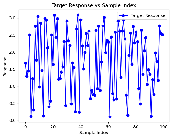
We can preview a plot of the response vector.
import matplotlib.pyplot as plt
plt.plot(response, label='Target Response', color='blue', marker="o")
plt.xlabel('Sample Index')
plt.ylabel('Response')
plt.title('Target Response vs Sample Index')
plt.legend()
plt.show()
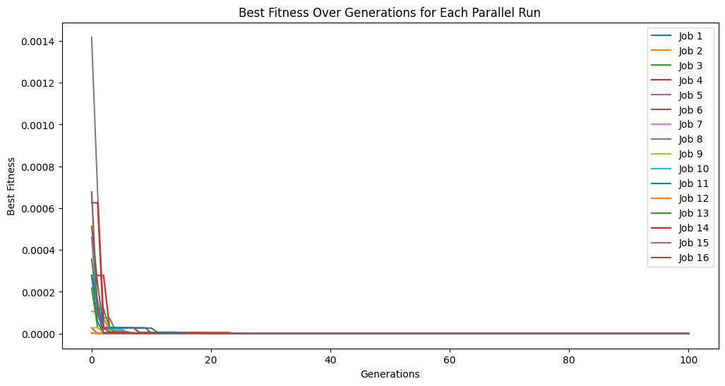
Now we can test the ability for StackGP to rediscover the target model using the benchmark data.
models = sgp.parallelEvolve(inputData,response,tracking=True)
Running parallel evolution with 16 jobs.
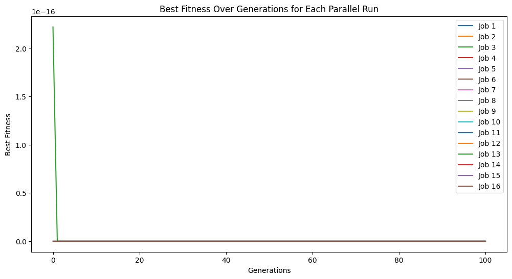
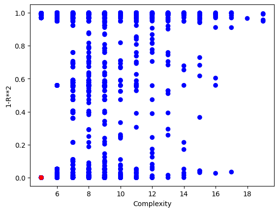
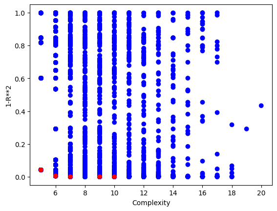
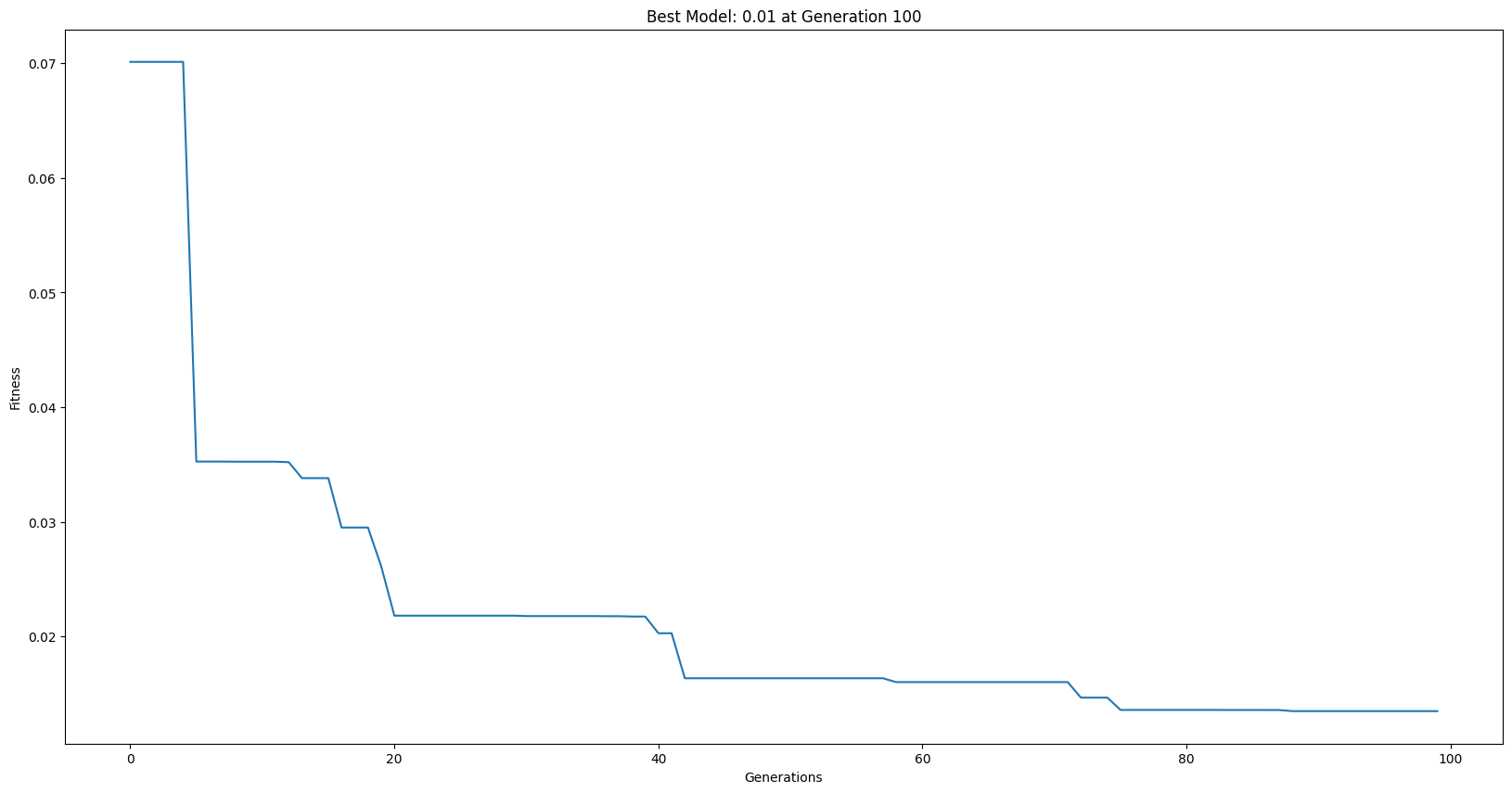
We can plot the model population to see the quality of the population. It looks like there are some models that are very simple and accurate.
sgp.plotModels(models)
Now we can check the symbolic form of the best model to see if it matches the generating function.
sgp.printGPModel(models[0])
Options#
This section showcases how each of the different arguments can be used with the generateRandomBenchmark function.
numVars: Controlling number of variables#
We can change the number of features in the data set and the max number of features allowed in the model using numVars.
In this example lets decrease the number of variables down to 1.
inputData, response, targetModel = sgp.generateRandomBenchmark(numVars=1)
sgp.printGPModel(targetModel)
We could also greatly increase the number of variables. For example to 50.
inputData, response, targetModel = sgp.generateRandomBenchmark(numVars=50)
sgp.printGPModel(targetModel)
If we want to increase the number of variables in use in the model while increasing the number of variables in the data, we would also need to increase the max allowed complexity of the model. For example, here we increase the number of variables to 50 and the max size of the model to 30.
inputData, response, targetModel = sgp.generateRandomBenchmark(numVars=50, maxLength=30)
sgp.printGPModel(targetModel)
This makes for a very challenging benchmark problem.
models = sgp.parallelEvolve(inputData,response,tracking=True)
Running parallel evolution with 16 jobs.
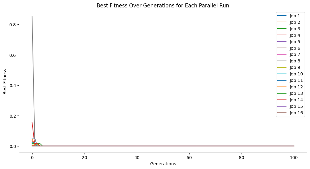
sgp.printGPModel(models[0])
numSamples: Controlling Number of Data Samples#
We may want to change the number of data samples in the benchmark. Sometimes we may want very small datasets to see if our ML method can efficiently utilize the data. Sometime we want to use large datasets to test the efficiency of using a lot of data. Other times, a problem may be so challenging that we just need a ton of data.
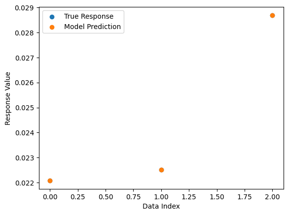
In this example below we decrease the number of samples to just 3 points and then try to find a model with those points.
inputData, response, targetModel = sgp.generateRandomBenchmark(numSamples=3)
sgp.printGPModel(targetModel)
# train models
models = sgp.parallelEvolve(inputData,response,tracking=True)
Running parallel evolution with 16 jobs.
# plot models
sgp.plotModels(models)
# print the best model found
sgp.printGPModel(models[0])
# plot the model prediction vs the target response
sgp.plotModelResponseComparison(models[0], inputData, response)
Here we increase the data set size to 10,000 to test the efficiency of our balancedSample strategy.
inputData, response, targetModel = sgp.generateRandomBenchmark(numSamples=10000)
sgp.printGPModel(targetModel)
models = sgp.evolve(inputData, response, liveTracking=True, liveTrackingInterval=0, dataSubsample=True, samplingMethod=sgp.balancedSample)
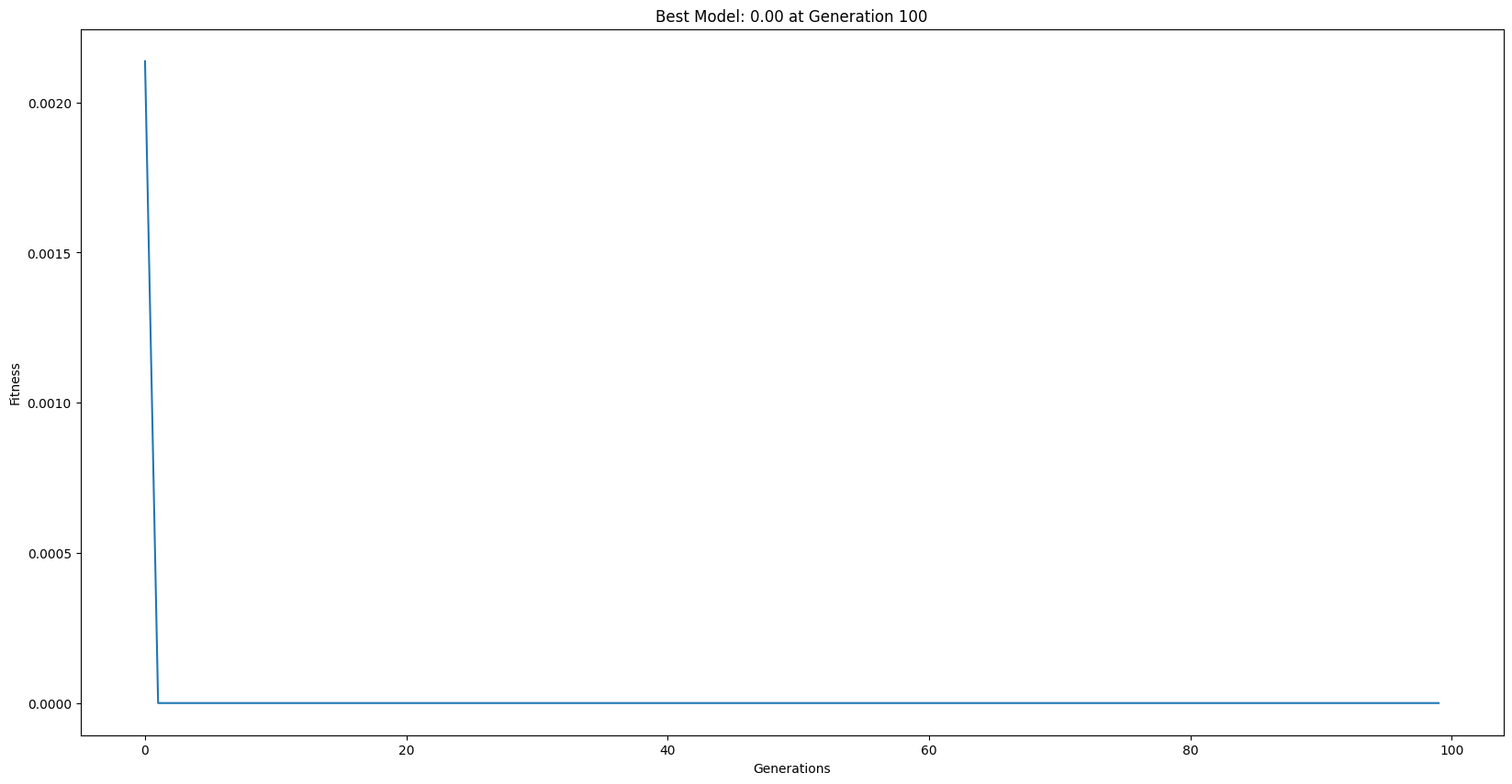
sgp.printGPModel(models[0])
noiseLevel: Controlling amount of noise.#
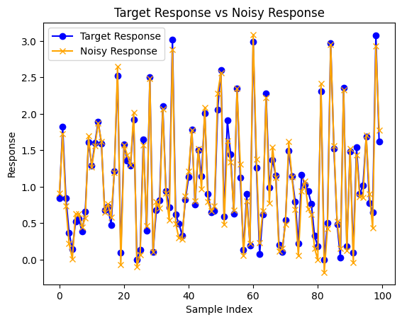
We may want to inject noise into the benchmark data to make it more challenging to rediscover the benchmark model as well as to assess the ML method’s sensitivity to noise. We can do this by modifying the noiseLevel argument.
In this example we increase the noise level to 10.
inputData, response, targetModel = sgp.generateRandomBenchmark(noiseLevel=0.1)
sgp.printGPModel(targetModel)
Now we can observe the difference between the truth model output and the noise corrupted output generated.
import matplotlib.pyplot as plt
truthResponse = sgp.evaluateGPModel(targetModel, inputData)
plt.plot(truthResponse, label='Target Response', color='blue', marker="o")
plt.plot(response, label='Noisy Response', color='orange', marker="x")
plt.xlabel('Sample Index')
plt.ylabel('Response')
plt.title('Target Response vs Noisy Response')
plt.legend()
plt.show()
models = sgp.parallelEvolve(inputData,response,tracking=True)
Running parallel evolution with 16 jobs.
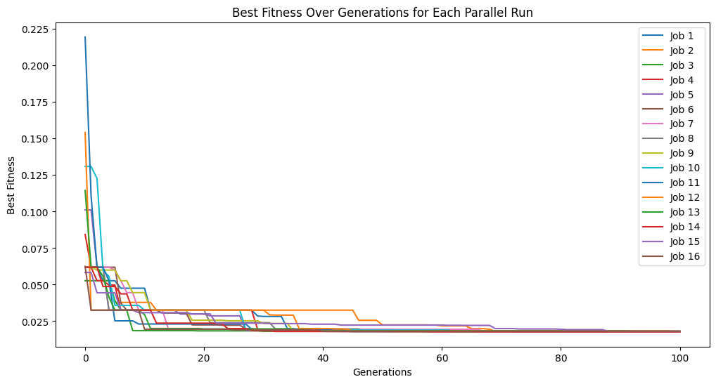
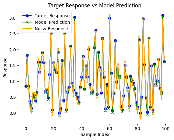
sgp.printGPModel(models[0])
predictedResponse = sgp.evaluateGPModel(models[0], inputData)
plt.plot(truthResponse, label='Target Response', color='blue', marker="o")
plt.plot(predictedResponse, label='Model Prediction', color='green', marker="x")
plt.plot(response, label='Noisy Response', color='orange', marker=".")
plt.xlabel('Sample Index')
plt.ylabel('Response')
plt.title('Target Response vs Model Prediction')
plt.legend()
plt.show()
opsChoices#
We may want to control the operators available in the model by either controlling for a specific set or expanding to a broader set to make search more difficult.
In this first example, we make the set more specific to just addition and subtraction.
inputData, response, targetModel = sgp.generateRandomBenchmark(opsChoices=[sgp.add, sgp.sub])
sgp.printGPModel(targetModel)
Maybe we want to expand to the full operator set in StackGP using sgp.allOps()
inputData, response, targetModel = sgp.generateRandomBenchmark(opsChoices=sgp.allOps())
sgp.printGPModel(targetModel)
Maybe we are interested in benchmarking a system with very specific operators. Here we generate a benchmark with just +, *, and sin.
inputData, response, targetModel = sgp.generateRandomBenchmark(opsChoices=[sgp.add, sgp.mult, sgp.sin])
sgp.printGPModel(targetModel)
constChoices#
We can supply a list of specific constants if we know that a specific set of constants will be useful. Note, that other constants can appear via combinations of the constants in the supplied set.
inputData, response, targetModel = sgp.generateRandomBenchmark(constChoices=[1,5,10])
sgp.printGPModel(targetModel)
Maybe we are interested in just having integer values
inputData, response, targetModel = sgp.generateRandomBenchmark(constChoices=[sgp.randomInt])
sgp.printGPModel(targetModel)
maxLength#
To make more complex problems we can increase the maxLength. To make a simpler problem, we can make smaller models using a smaller maxLength.
In the first example we decrease the length to 1, which means a model can have at most 1 operator.
inputData, response, targetModel = sgp.generateRandomBenchmark(maxLength=1)
sgp.printGPModel(targetModel)
We can drastically increase this value to get much more complicated models. Here we increase it to 100. Note: maxLength is a maximum value, so simpler model can still be returned.
inputData, response, targetModel = sgp.generateRandomBenchmark(maxLength=100)
sgp.printGPModel(targetModel)
seed: For Reproducibility#
We may want to be able to reproduce the same example rather than generating a new example every time. We can do this by setting the seed argument.
In this example we will show how setting the seed controls the output. In the first example, we don’t set a seed.
inputData, responseData, benchmarkModel = sgp.generateRandomBenchmark()
sgp.printGPModel(benchmarkModel)
Now if we run the same code below, we will likely get a different model.
inputData, responseData, benchmarkModel = sgp.generateRandomBenchmark()
sgp.printGPModel(benchmarkModel)
Now if we set the seed=10 we can see that we get the same result every time.
inputData, responseData, benchmarkModel = sgp.generateRandomBenchmark(seed=10)
sgp.printGPModel(benchmarkModel)
inputData, responseData, benchmarkModel = sgp.generateRandomBenchmark(seed=10)
sgp.printGPModel(benchmarkModel)
Examples#
This section some neat examples using the generateRandomBenchmark function.
Setting up a benchmark problem to test performance of serial vs parallel evolutionary search#
Here we generate a benchmark to see how much performance gain we get when using parallel search over serial search.
inputData, response, targetModel = sgp.generateRandomBenchmark()
sgp.printGPModel(targetModel)
Now lets split the data into training and testing data.
trainInput = inputData[:,:50]
trainResponse = response[:50]

testInput = inputData[:, 50:]
testResponse = response[50:]
First lets run the serial evolutionary search.
serialModels = sgp.evolve(trainInput, trainResponse, liveTracking=True, liveTrackingInterval=0)
Now lets run a parallel search using the same parameters.
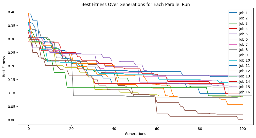
parallelModels = sgp.parallelEvolve(inputData, response, tracking=True)
Running parallel evolution with 16 jobs.
** On entry to DLASCL, parameter number  4 had an illegal value
** On entry to DLASCL, parameter number  4 had an illegal value
** On entry to DLASCL, parameter number  4 had an illegal value
** On entry to DLASCL, parameter number  5 had an illegal value
** On entry to DLASCL, parameter number  4 had an illegal value
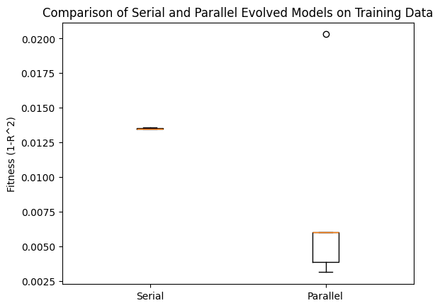
Now lets compare the best 10 models from both searches with respect to the training data.
serialTrainPerformance = [sgp.fitness(model, trainInput, trainResponse) for model in serialModels[:10]]
parallelTrainPerformance = [sgp.fitness(model, trainInput, trainResponse) for model in parallelModels[:10]]
# Plotting the boxplot to compare the two sets of performance
plt.boxplot([serialTrainPerformance, parallelTrainPerformance], labels=['Serial', 'Parallel'])
plt.ylabel('Fitness (1-R^2)')
plt.title('Comparison of Serial and Parallel Evolved Models on Training Data')
plt.show()
/var/folders/tn/s_jbjrf525zd165vpvwykqk40000gn/T/ipykernel_3951/1328465278.py:4: MatplotlibDeprecationWarning: The 'labels' parameter of boxplot() has been renamed 'tick_labels' since Matplotlib 3.9; support for the old name will be dropped in 3.11.
  plt.boxplot([serialTrainPerformance, parallelTrainPerformance], labels=['Serial', 'Parallel'])
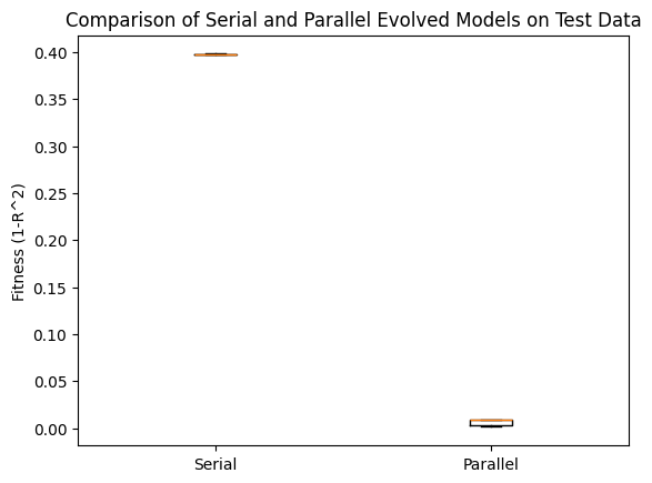
Now we can check the same comparison using the test data. We can see that the parallel search performed MUCH better.
serialTestPerformance = [sgp.fitness(model, testInput, testResponse) for model in serialModels[:10]]
parallelTestPerformance = [sgp.fitness(model, testInput, testResponse) for model in parallelModels[:10]]
# Plotting the boxplot to compare the two sets of performance
plt.boxplot([serialTestPerformance, parallelTestPerformance], labels=['Serial', 'Parallel'])
plt.ylabel('Fitness (1-R^2)')
plt.title('Comparison of Serial and Parallel Evolved Models on Test Data')
plt.show()
/var/folders/tn/s_jbjrf525zd165vpvwykqk40000gn/T/ipykernel_3951/854879436.py:4: MatplotlibDeprecationWarning: The 'labels' parameter of boxplot() has been renamed 'tick_labels' since Matplotlib 3.9; support for the old name will be dropped in 3.11.
  plt.boxplot([serialTestPerformance, parallelTestPerformance], labels=['Serial', 'Parallel'])
Now we can look at the forms of the best models from both the serial search and parallel search.
sgp.printGPModel(serialModels[0])
sgp.printGPModel(parallelModels[0])
We can compare to the ground truth model form below.
sgp.printGPModel(targetModel)