StackGP.parallelEvolve#
StackGP.parallelEvolve(inputData, responseData, n_jobs=-1, avail_cores=-1, cascades=False, cascadeCount=10, exchangeCount=5, **kwargs)
ParallelEvolve is the core search engine within StackGP parallelized to runs multiple evolutions at the same time.
In the minimal use case, you need to supply and input dataset and a response vector to fit. All arguments available for the Evolve function are also available for the ParallelEvolve Function.
There are a few additonal arguments available to parallelEvolve that aren’t available in evolve:
n_jobs: The number of parallel jobs to run. Default=-1, which uses all available cores.
avail_cores: The number of cores available. By default StackGP attempts to identify all cores available, but there may be cases where you want to control this. The default avail_cores=-1, will attempt to use all available cores.
cascades: A boolean flag that controls whether multiple cascades shuold be run or not. By default this is set to False.
cascadeCount: The number of cascades (evolutionary epochs) to complete. When cascades=True, the default is 10.
exchangeCount: The number of random models to exchange between parallel populations between cascades. The default is set to 5.
First we need to load in the necessary packages
import StackGP as sgp
import numpy as np
Overview#
Define Function#
Here we define the function and data which we will try to rediscover.
#Define demo function to generate data
inputData, response, targetModel = sgp.generateRandomBenchmark()
sgp.printGPModel(targetModel)
GP Search#
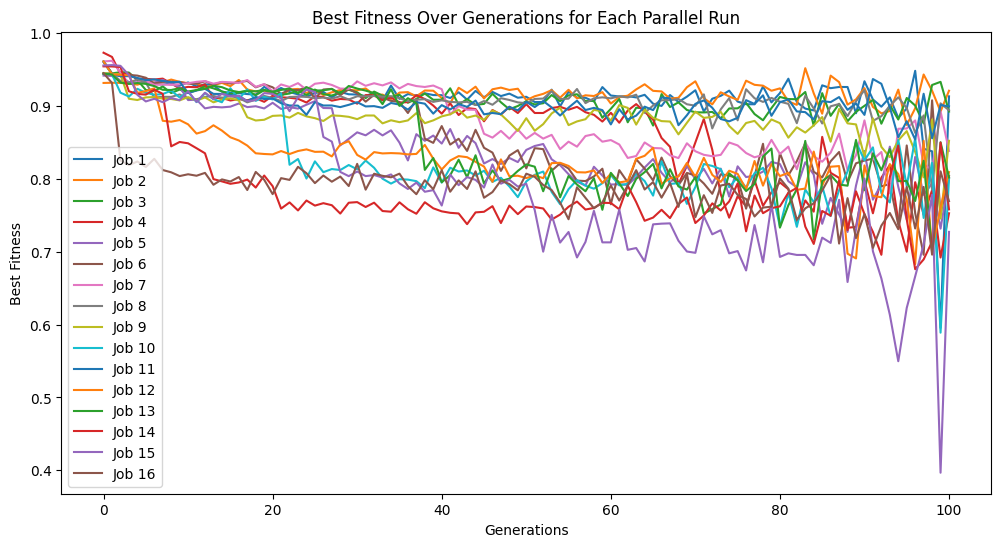
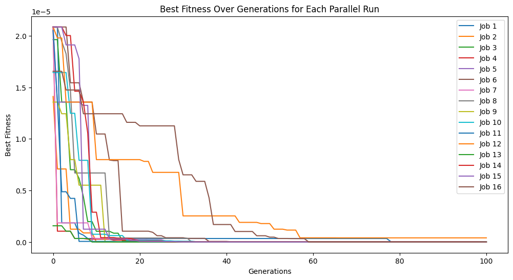
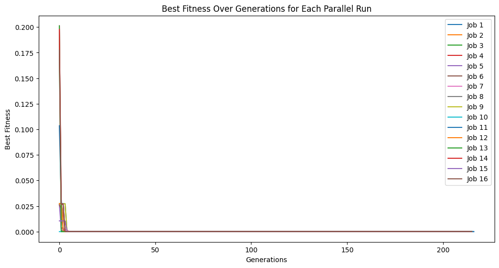
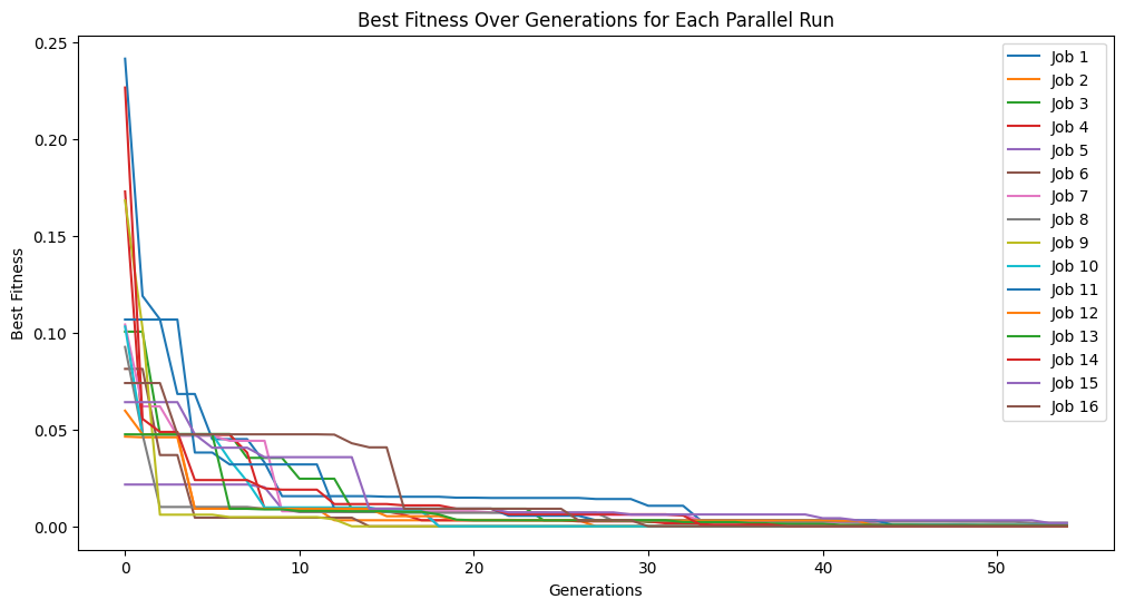
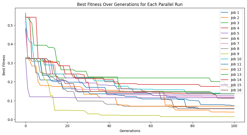
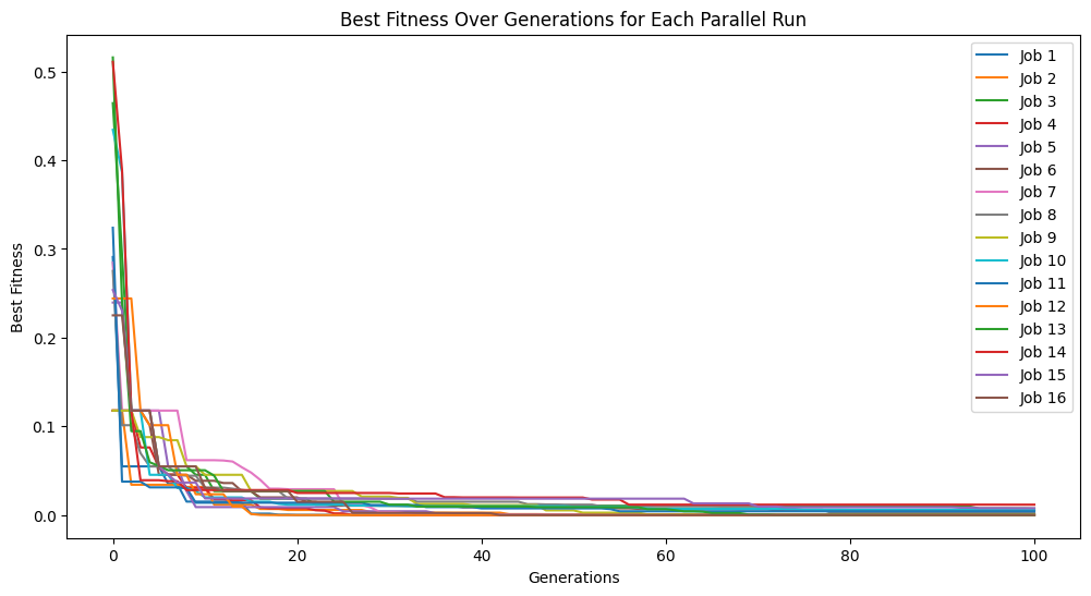
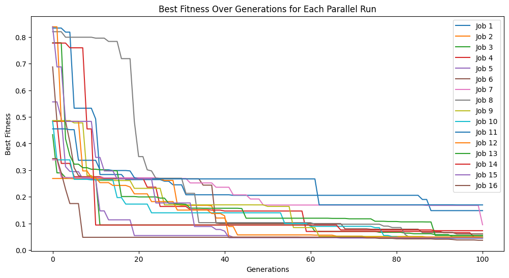
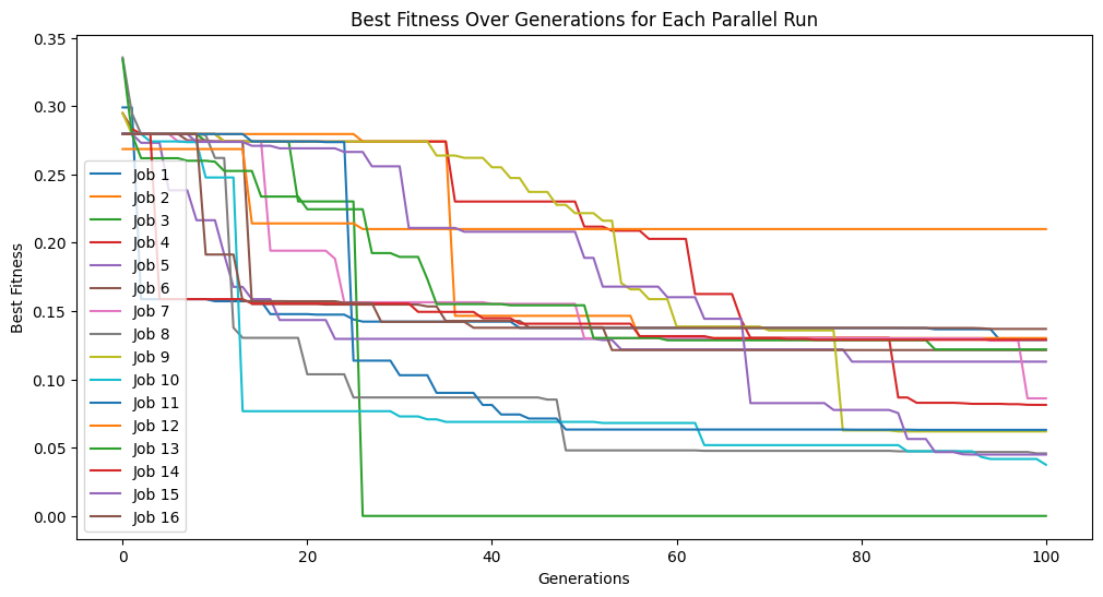
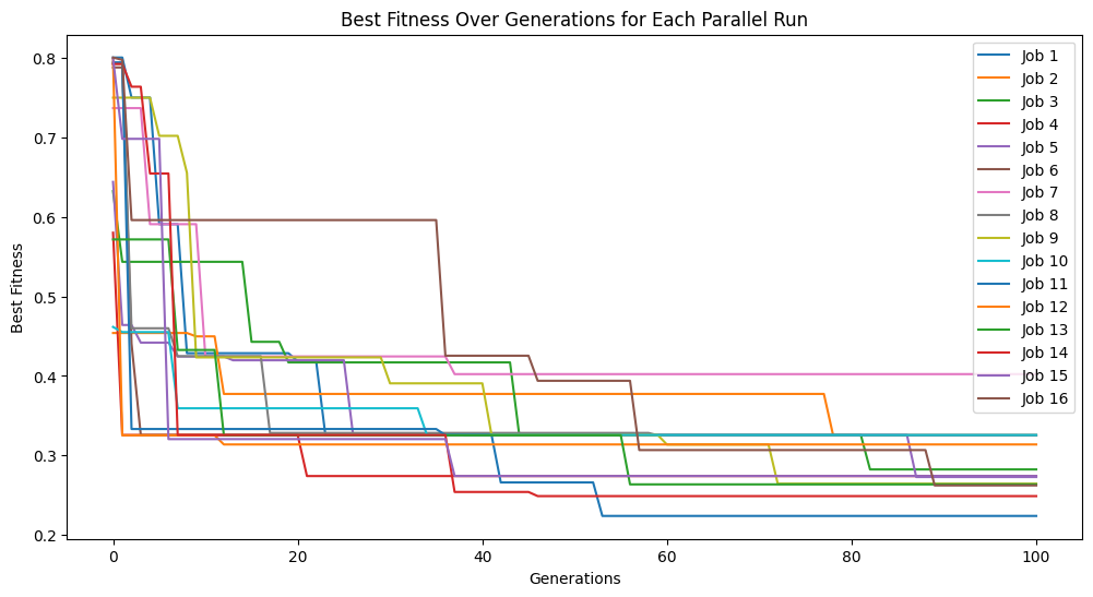
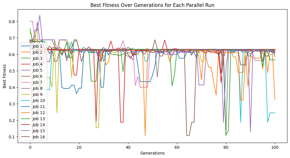
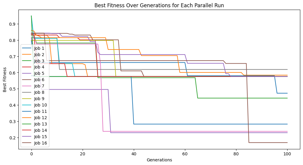
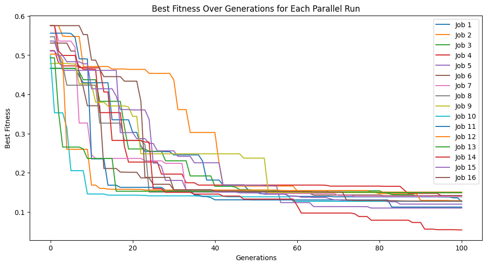
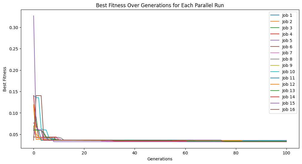
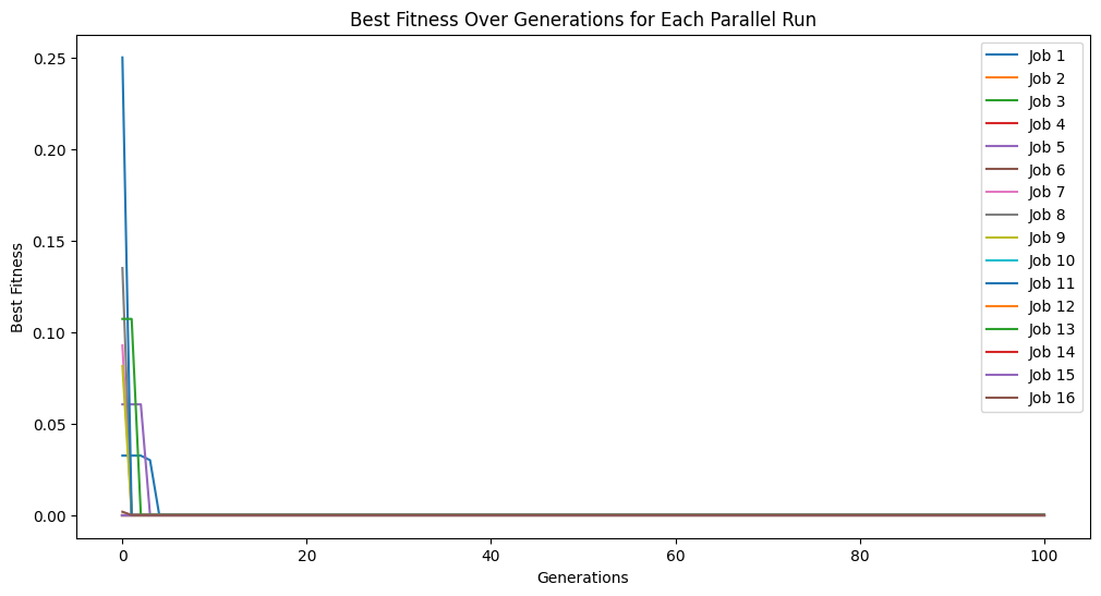
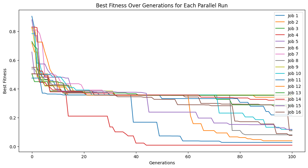
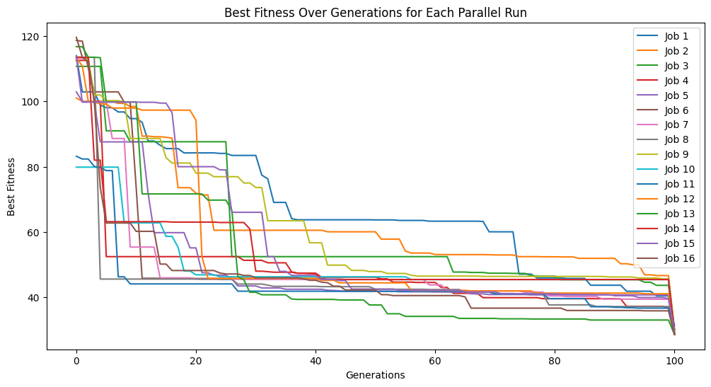
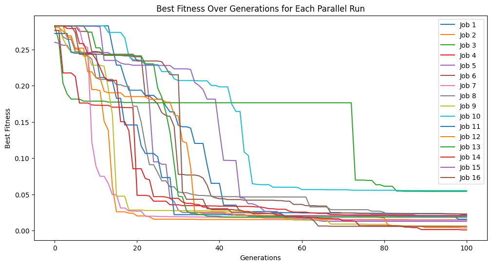
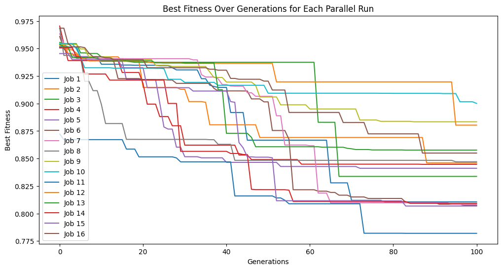
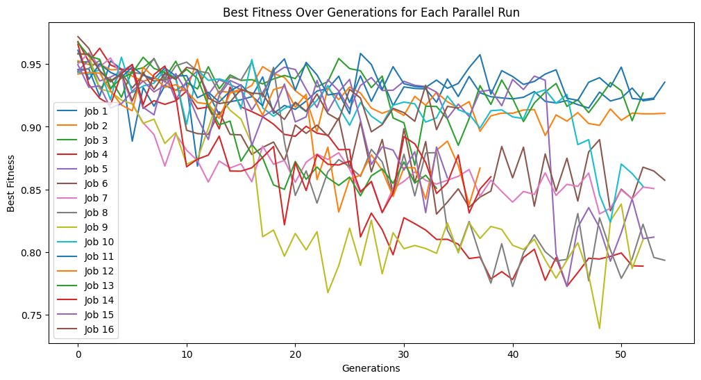
Here we supply the input data and response to StackGP’s parallelEvolve function to search for a model that fits the data. To visualize the peformance across all the runs, we have enabled tracking=True.
#Generate models
models=sgp.parallelEvolve(inputData,response,tracking=True)
Running parallel evolution with 16 jobs.
Results#
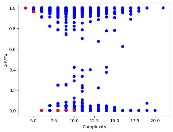
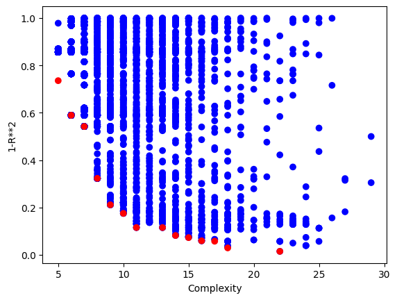
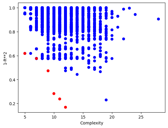
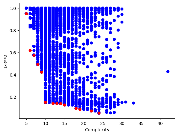
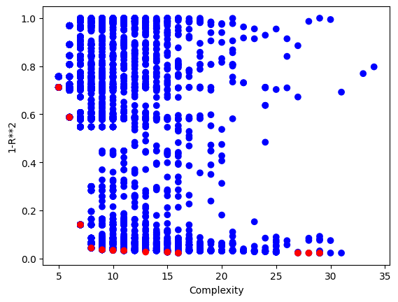
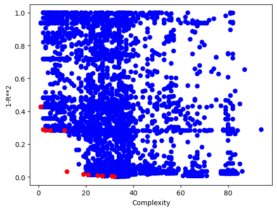
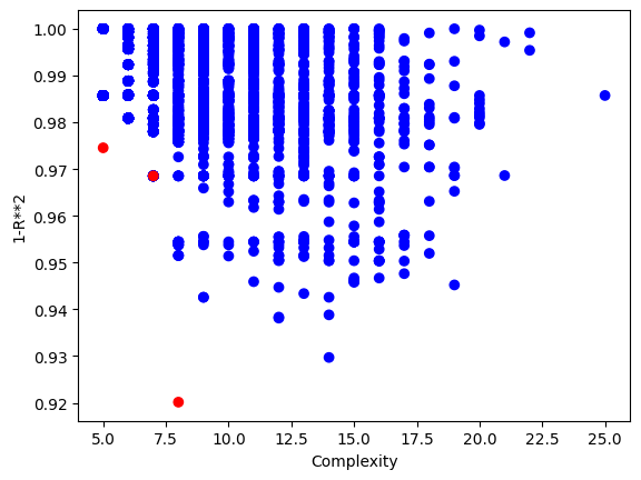
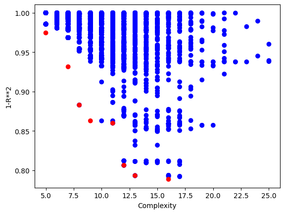
Now we can visualize the Pareto front plot of the evolved models to see how they perform with respect to accuracy and complexity. Compared to using the serial evolve function, we can see that a lot more models are returned.
#View model population quality
sgp.plotModels(models)
We can use the printGPModel function to print the best model in a readable format.
#View best model
sgp.printGPModel(models[0])
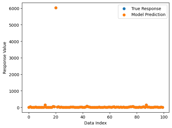
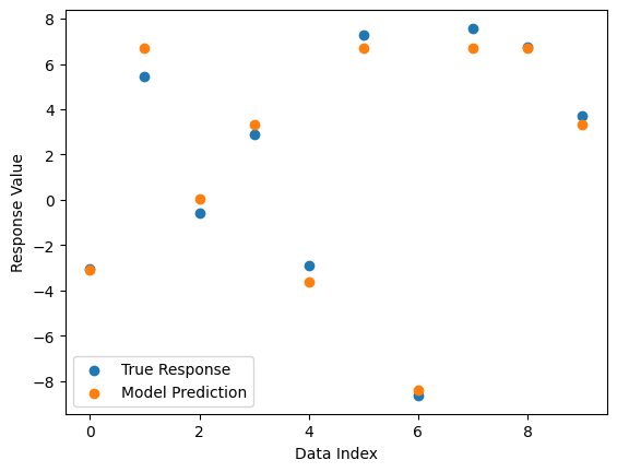
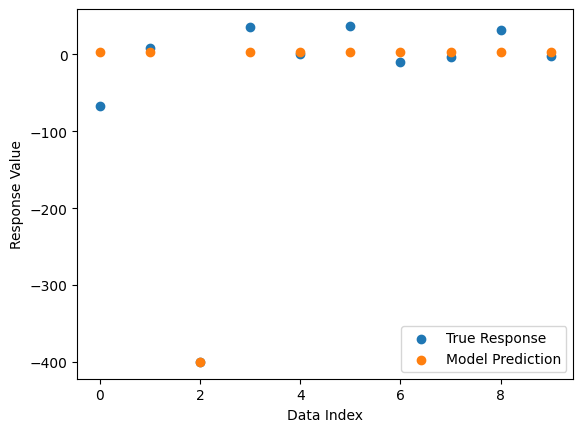
We can also plot a comparison between predicted and observed values.
#Compare best model prediction to true data
sgp.plotModelResponseComparison(models[0],inputData,response)
Options#
This section showcases how each of the different option settings can be used with the parallelEvolve function. First we will showcase the two options specific to parallelEvolve (n_jobs and avail_cores) before providing examples for options available to parallelEvolve as well as evolve.
n_jobs#
n_jobs can be used to specify how many parallel runs we want to execute. If n_jobs is less than avail_cores, jobs will run in parallel. If n_jobs is greater than avail_cores, jobs will run in batches.
First lets setup a random benchmark dataset to showcase the algorithm.
inputData, response, targetModel = sgp.generateRandomBenchmark()
sgp.printGPModel(targetModel)
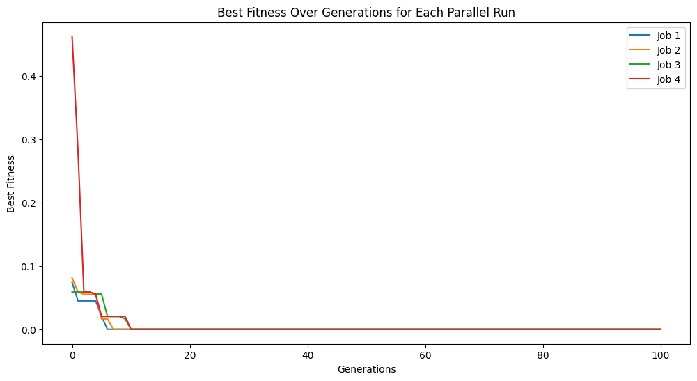
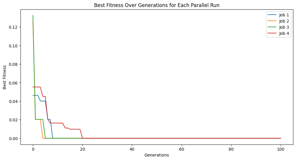
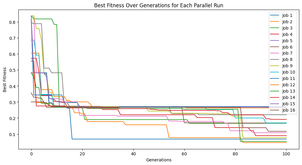
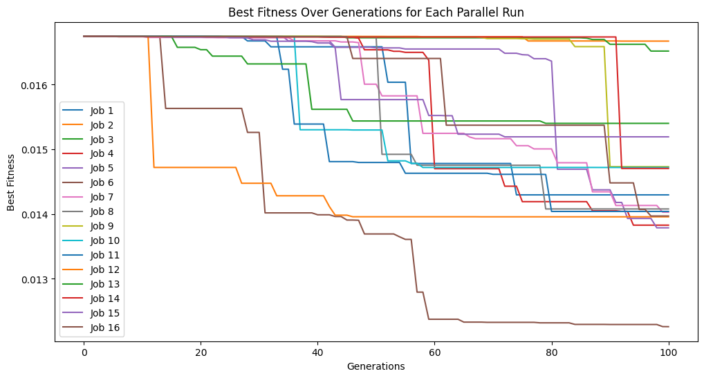
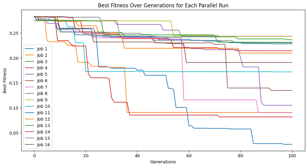
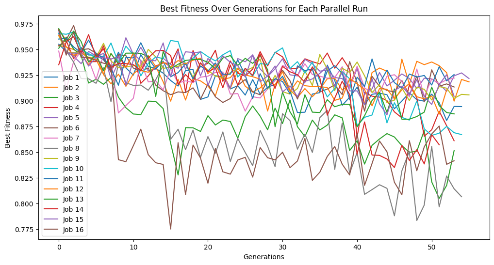
Now lets setup an evolutionary search using just 4 cores. We can see the evolutionary traces of the 4 runs in the plot since we have tracking=True.
models = sgp.parallelEvolve(inputData, response, tracking=True, n_jobs=4)
Running parallel evolution with 4 jobs.
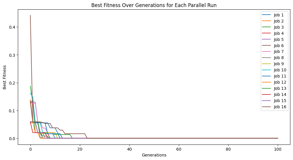
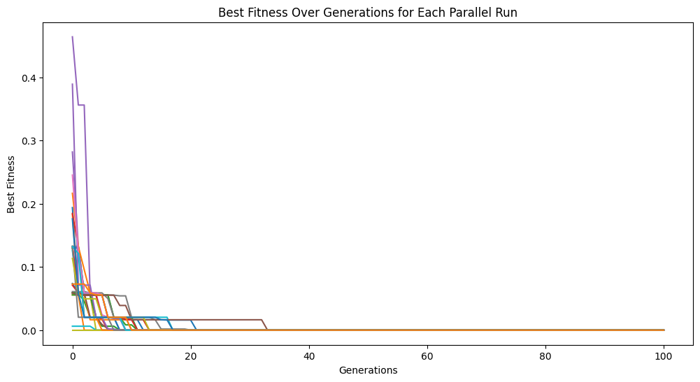
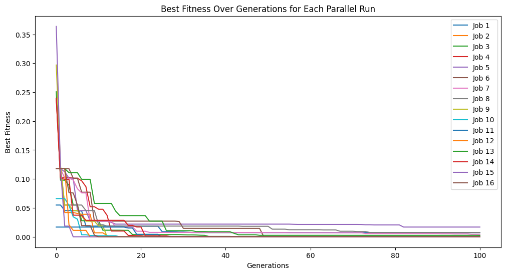
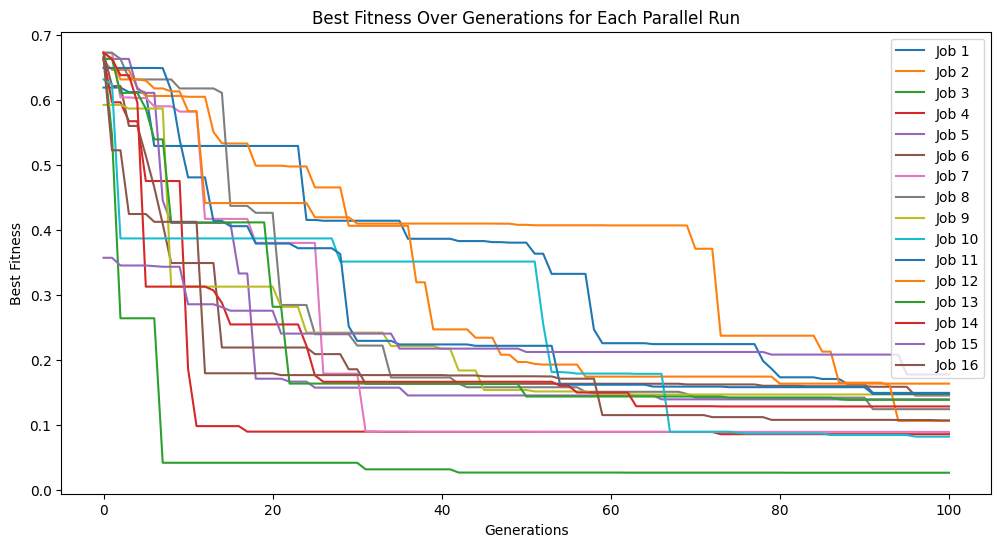
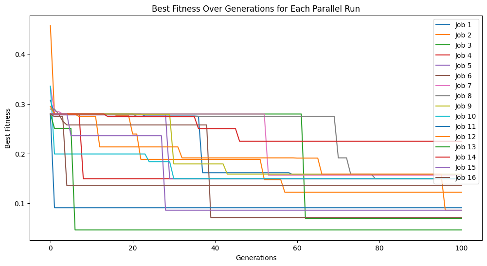
Now lets compare to setting n_jobs=-1 so that it uses all available cores.
models = sgp.parallelEvolve(inputData,response,tracking=True, n_jobs=-1)
Running parallel evolution with 16 jobs.
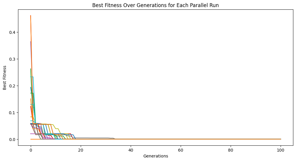
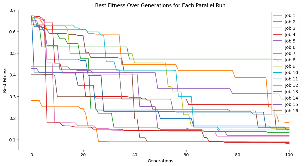
Now we can see what happens when we use more jobs than there are cores. In this case, we will use 32 which is twice as many jobs as we have cores. This will take twice as long to run since it runs in two batches.
models = sgp.parallelEvolve(inputData,response,tracking=True, n_jobs=32)
Running parallel evolution with 32 jobs.
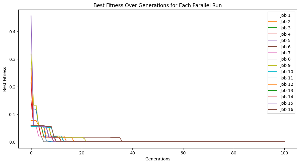
If we don’t want to use all cores at once, for example if running on an HPC system where you should not be using all available cores at once, we can limit the number of cores and run the jobs in batches by having a smaller number of available cores than jobs.
models = sgp.parallelEvolve(inputData,response,tracking=True, n_jobs=16, avail_cores=4)
Running parallel evolution with 16 jobs.
avail_cores#
There may be cases where either the automated detection of cores fails or you do not actually want to use all the available cores. For example, if you are using a shared HPC resource, you may not want to monopolize the system. In this case, you can manually set the number of available cores using avail_cores.
In this case, we will reduce the number of available cores to 4.
models = sgp.parallelEvolve(inputData,response,tracking=True, avail_cores=4, n_jobs=4)
Running parallel evolution with 4 jobs.
Interestingly, we can also increase the number of cores above what is detected by StackGP or even what is physically available on the system. This is likely not a good practice though unless your system supports hyperthreading or you are certain the number of detected cores is wrong.
models = sgp.parallelEvolve(inputData,response,tracking=True, avail_cores=32, n_jobs=32)
Running parallel evolution with 32 jobs.
cascades#
cascades is a boolean option that controls if multiple evolutionary epochs should be run in sequence and in parallel. Between cascades, models can be exchanged between the independent populations if exchangeCount is greater than 0. Some research in the field of evolutionary computing has shown this strategy to be beneficial.
First lets generate a benchmark problem to use in this example.
inputData, response, targetModel = sgp.generateRandomBenchmark()
sgp.printGPModel(targetModel)
Below, we set cascades=True and cascadeCount=5 to run through 5 evolutionary epochs. We also enabled liveTracking but note that the updates in the figure can only occur between cascades when results are returned to the main kernel.
cascadeModels = sgp.parallelEvolve(inputData, response, liveTracking=True, cascades=True, cascadeCount=5)
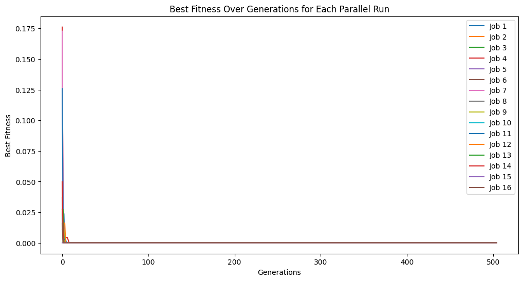
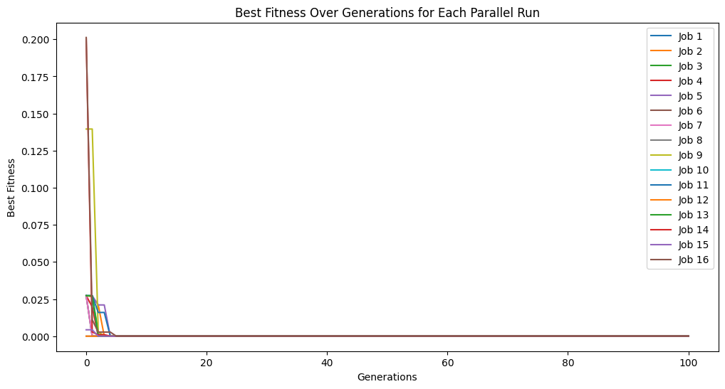
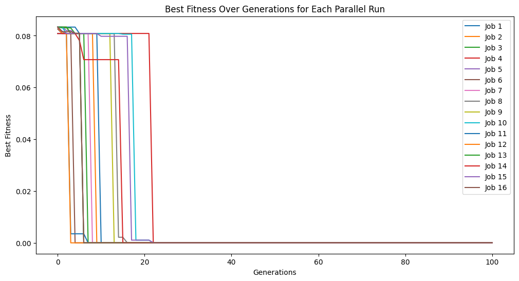
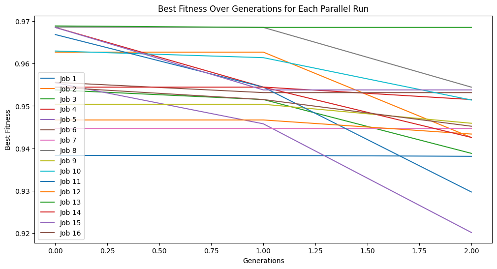
Below, we disable cascades. Compared to the previous example, we can see that we only get through 100 generations rather than the 500 we got from running through 5 cascades.
noCascadeModels = sgp.parallelEvolve(inputData, response, liveTracking=True, tracking=True, cascades=False)
Running parallel evolution with 16 jobs.
Live tracking is not supported in parallel evolution without cascades, disabling live tracking.
When using a timeLimit with capTime=True the time limit is enforced over the total of all cascades rather than per cascade. Thus, if timeLimit=30 (30 seconds), regardless of how many cascades are set, the runtime will be capped at 30 seconds. We can see this below. Despite setting cascades to 10, we only get through a few in the 30 seconds. As well, the time limit will interrupt an in progress cascade and return the models at that point.
cascadesTimeLimitModels = sgp.parallelEvolve(inputData, response, liveTracking=True, cascades=True, cascadeCount=10, capTime=True, timeLimit=30)
cascadeCount#
cascadeCount can be used to control how many cascades are completed if cascades=True.
inputData, response, targetModel = sgp.generateRandomBenchmark()
sgp.printGPModel(targetModel)
Below we show an example where we complete 5 cascades where we use 50 generations in each cascade.
cascade5Models = sgp.parallelEvolve(inputData, response, liveTracking=True, generations=50, cascades=True, cascadeCount=5)
Below we show another example where we increase the number of cascades to 20 but decrease the generations per cascade to just 10.
cascade20Models = sgp.parallelEvolve(inputData, response, liveTracking=True, generations=10, cascades=True, cascadeCount=20)
exchangeCount#
exchangeCount can be used to control how many models are randomly exchanged between independent populations between each cascade. When this is set to a value greater than 0, each population sends the set exchangeCount individuals to a random other population. This allows some information to be exchanged between populations while still allowing each population to develop somewhat independently.
inputData, response, targetModel = sgp.generateRandomBenchmark()
sgp.printGPModel(targetModel)
Below we set exchangeCount=0 meaning there is no exchange of individuals between populations. In this case, we see each population progressing entirely independently.
exchange0Models = sgp.parallelEvolve(inputData, response, liveTracking=True, tracking=True, generations=10, cascades=True, cascadeCount=5, exchangeCount=0)
Below we set exchangeCount=5 which allows 5 models to be randomly exchanged between populations after each cascade. This allows some beneficial genetic information to flow between populations while still allowing each population to have some independence. This can be observed by seeing the population traces a little closer together over multiple cascades.
exchange5Models = sgp.parallelEvolve(inputData, response, liveTracking=True, tracking=True, generations=10, cascades=True, cascadeCount=5, exchangeCount=5)
This effect is more pronounced if we exchange the entire population size between populations. Here we set the exchange count to 300 and we can see that the populations converge very quickly.
exchange100Models = sgp.parallelEvolve(inputData, response, liveTracking=True, tracking=True, generations=10, cascades=True, cascadeCount=5, exchangeCount=300)
generations#
generations can be used to control how many generations are used in search. The default is to use 100, but if the problem is difficult it may be beneficial to increase this.
First lets setup a somewhat challenging problem with nonlinear patterns. As well, we won’t include cosine, sine, or log in the search space, so we will have to find an approximate model.
#Define a challenging function to generate data
def demoFunc(x,y):
    return np.sin(x) * np.cos(y) + np.log(x + y)
#Generate data
inputData=np.array([np.random.randint(1,10,10),np.random.randint(1,10,10)])
response=demoFunc(inputData[0],inputData[1])
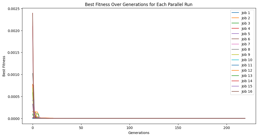
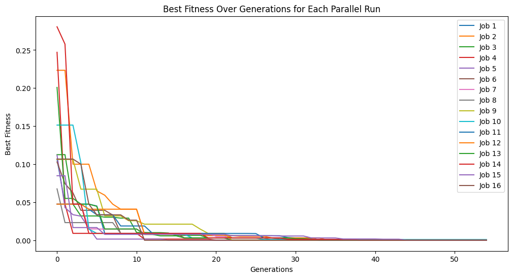
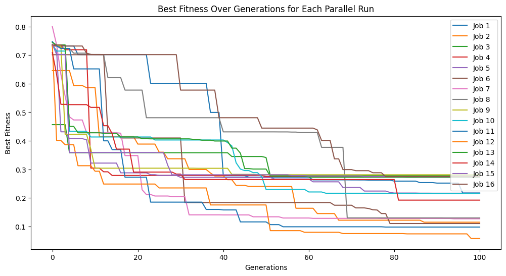
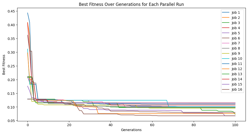
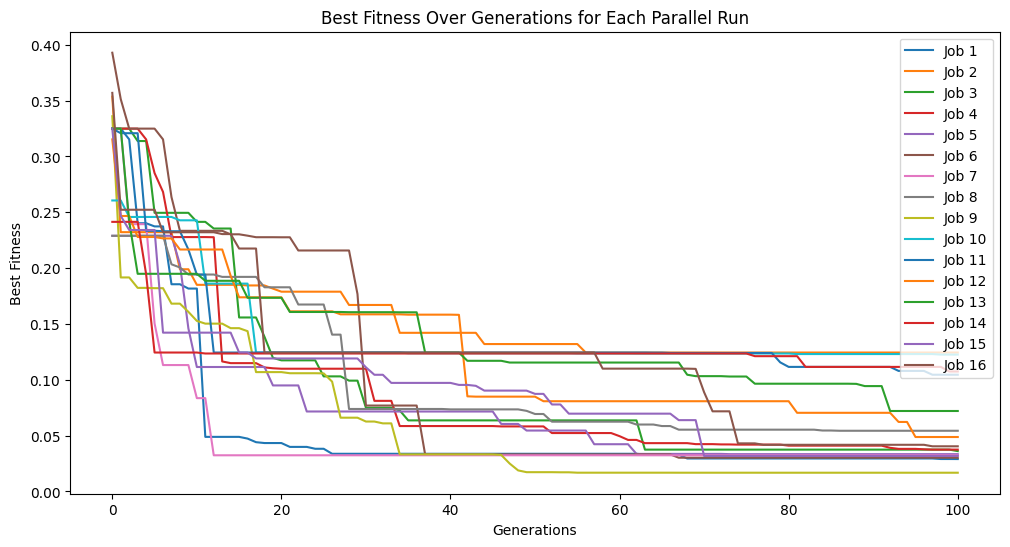
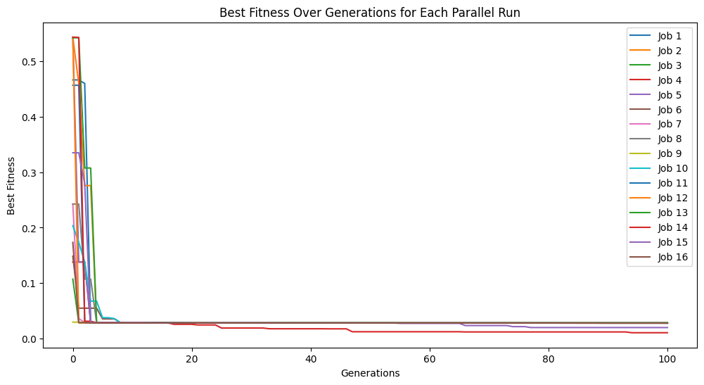
Now lets try fitting with the default settings. We will turn on tracking so we can see the progress.
#Generate models
models=sgp.parallelEvolve(inputData,response,tracking=True)
Running parallel evolution with 16 jobs.
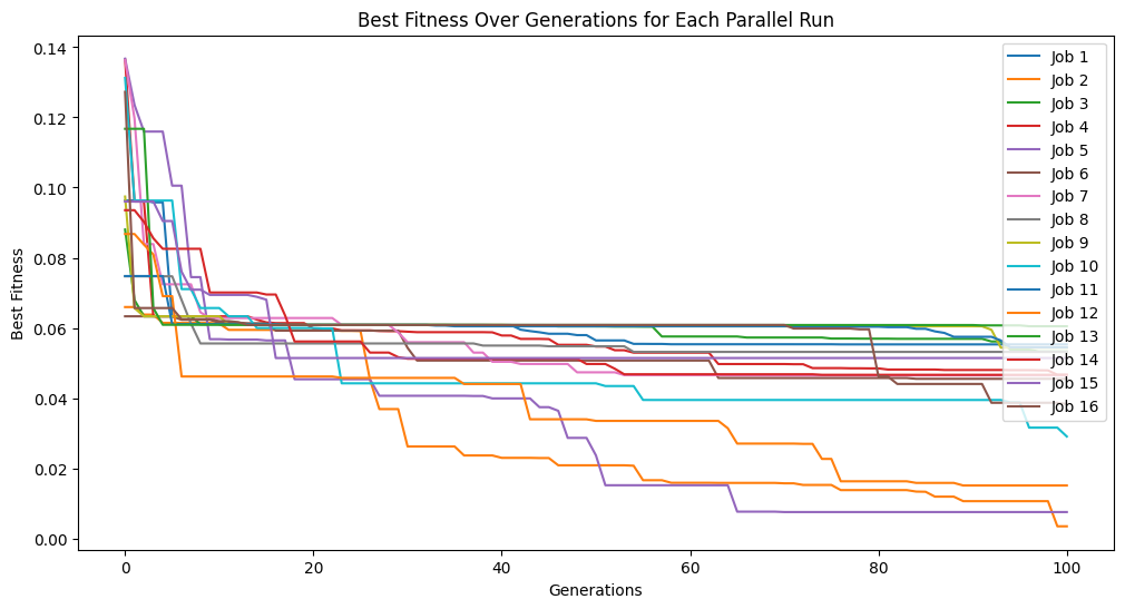
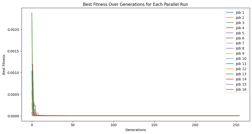
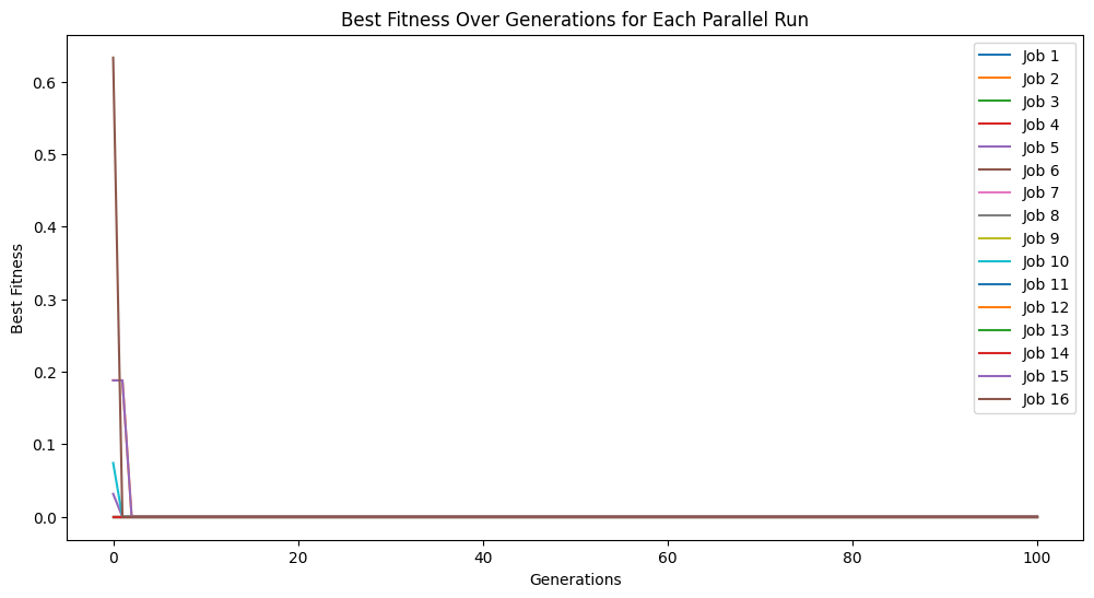
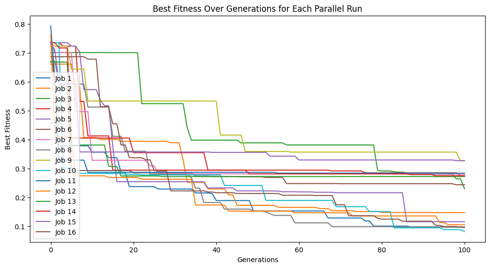
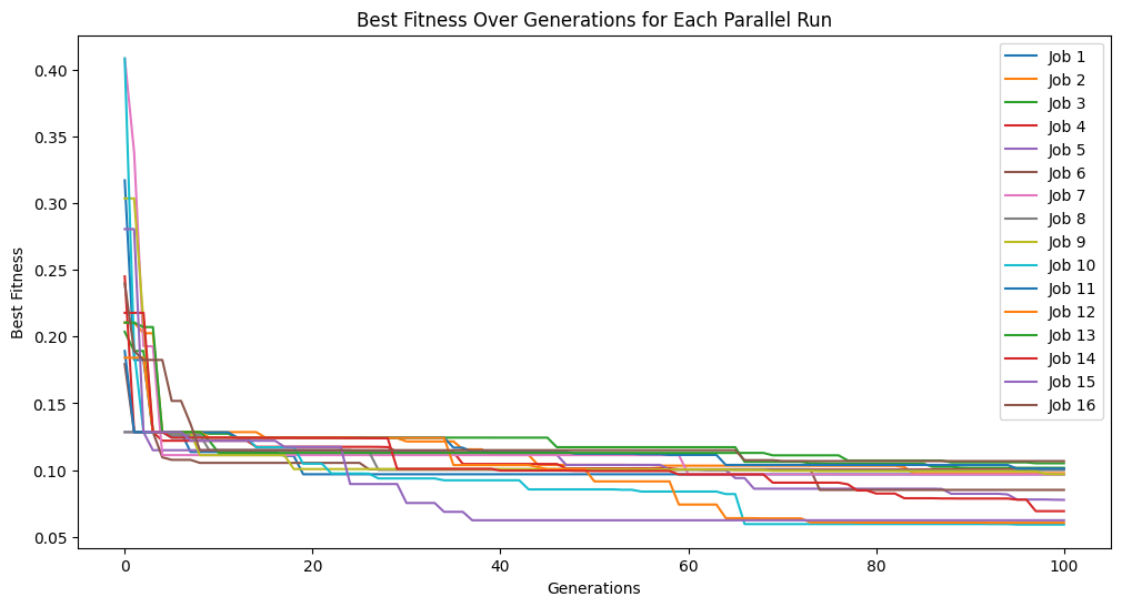
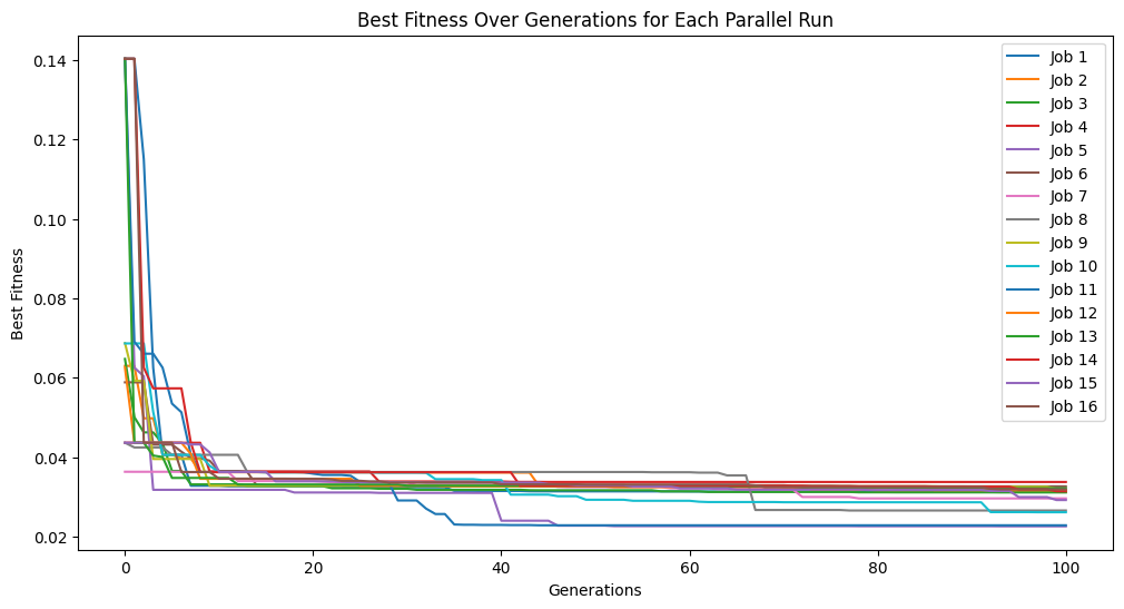
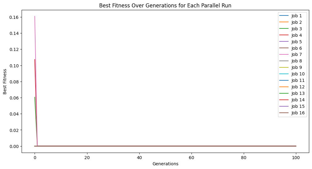
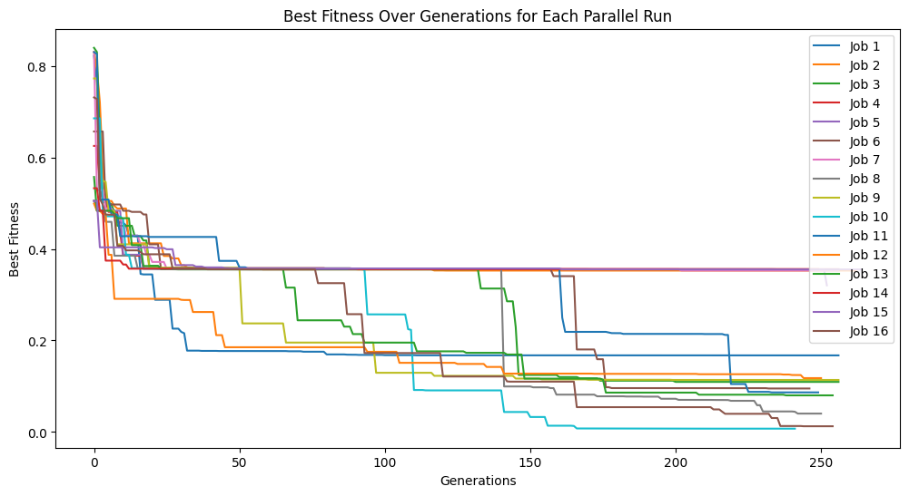
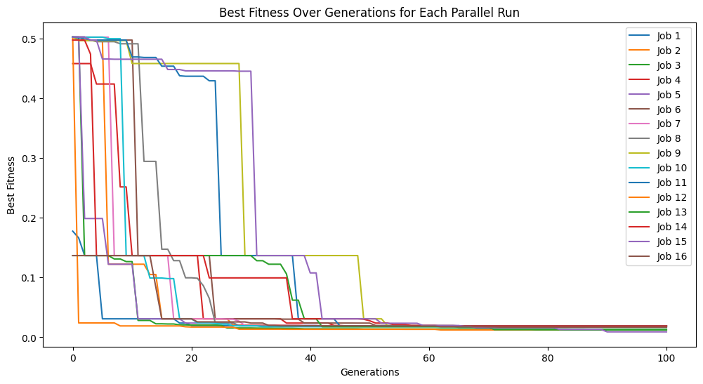
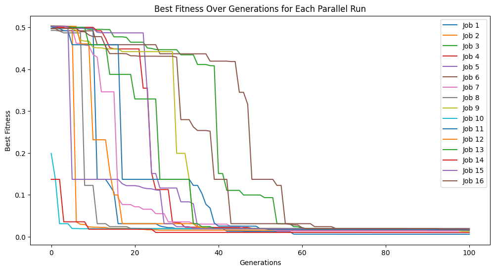
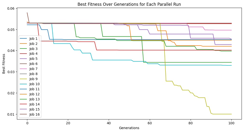
Now lets crank up the number of generations to see if we can get closer.
#Generate models
models=sgp.parallelEvolve(inputData,response,generations=1000,tracking=True)
Running parallel evolution with 16 jobs.
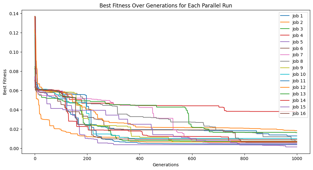
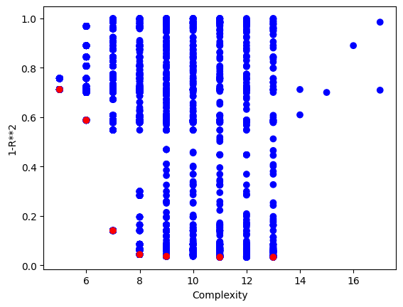
We can see that the extra generations allowed us to get a much better fitness score.
ops#
By default ops is set to defaultOps(), which contains: div, add, sub, mult, exp, sqrd, sqrt, and inv. These are generally good to try as a starting point since including too many terms or including highly nonlinear terms when they aren’t needed can lead to overfitting.
First lets demonstrate the default case on a problem where the operator set is not sufficient to find a perfect solution.
#Define a challenging function to generate data
def demoFunc(x,y):
    return np.sin(x) * y
#Generate data
inputData=np.array([np.random.randint(1,10,10),np.random.randint(1,10,10)])
response=demoFunc(inputData[0],inputData[1])
#Generate models
models=sgp.parallelEvolve(inputData,response,tracking=True)
Running parallel evolution with 16 jobs.
#Plot models
sgp.plotModels(models)
#View best model
sgp.printGPModel(models[0])
#Compare best model prediction to true data
sgp.plotModelResponseComparison(models[0],inputData,response)
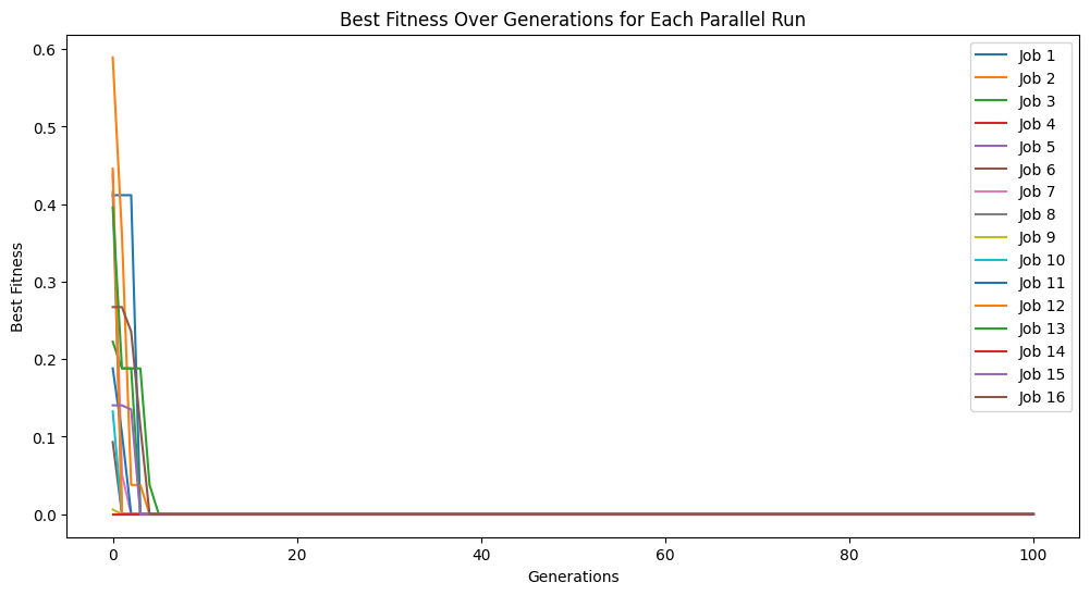
Now we set ops to allOps() which includes default set plus trig functions and log. This makes it possible to find an exactl solution.
#Generate models
models=sgp.parallelEvolve(inputData,response,ops=sgp.allOps(), tracking=True)
Running parallel evolution with 16 jobs.
#View best model
sgp.printGPModel(models[0])
We can see now that the solution was discovered.
const#
The const option allows for control over what constants are to be used when generating random models. The default settings of defaultConst() captures many commonly used constants, but there may be instances where these are not sufficient or domain knowledge can be used to provide a better set.
#Define a challenging function to generate data
def demoFunc(x,y):
    return np.pi*x / (np.pi/2 + y)
#Generate data
inputData=np.array([np.random.randint(1,10,10),np.random.randint(1,10,10)])
response=demoFunc(inputData[0],inputData[1])
#Generate models
models=sgp.parallelEvolve(inputData,response,tracking=True,ops=sgp.allOps(),const=sgp.defaultConst())
Running parallel evolution with 16 jobs.
#View best model
sgp.printGPModel(models[0])
In the above case, we can see that while we did get a good fitness, the search struggled to find the correct constants and resorted to do its best to approximate the data.
Below, we demonstrate that if we supply the search with good constants, we can make the search much easier. This example outlines and extreme scenario where we happen to know the correct constants. This is unlikely to occur in practice, but it provides good insight into how the constant set can impact search.
#Generate models
models=sgp.parallelEvolve(inputData,response,tracking=True,ops=sgp.allOps(),const=[np.pi, np.pi/2])
Running parallel evolution with 16 jobs.
#View best model
sgp.printGPModel(models[0])
We can see that we discovered the correct model in this case by supplying the correct constants.
variableNames#
By default, variables are named \(x1\), \(x2\), … Likely you will know the names of features in your dataset, so we can supply those to the search to build models with the supplied names to improve their interpretability.
#Define a function to generate data
def pressureFunc(temperature,volume):
    return temperature/volume
#Generate data
inputData=np.array([np.random.randint(1,10,10),np.random.randint(1,10,10)])
response=pressureFunc(inputData[0],inputData[1])
#Generate models
models=sgp.parallelEvolve(inputData,response,tracking=True)
Running parallel evolution with 16 jobs.
#View best model
from sympy import symbols
sgp.printGPModel(models[0],symbols(['temperature','volume']))
While the default case does find a model that perfectly fits the data, there is no reason to leave it to the user to interpret the default variable names and convert them to something informative. Rather, we can just supply them directly to the search. (Note: This is not fully supported yet to embed the feature names in evolution, but this is a placeholder for when it is supported. For now we can still see the interpretable form by supplying the names to printGPModel)
#Generate models
from sympy import symbols
models=sgp.parallelEvolve(inputData,response,tracking=True,ops=sgp.allOps(),variableNames=symbols(['temperature','volume']))
Running parallel evolution with 16 jobs.
#View best model
sgp.printGPModel(models[0],symbols(['temperature','volume']))
mutationRate#
We can control the percentage of model created in each generation from mutation by modifying the mutationRate. It may be the case that mutation is either better or worse suited for the problem than crossover or random generation of models, so we can tune this. The default setting should be reasonably robust, so it is not expected that you will have to modify this setting. As well, evolutionary search tends to be pretty robust to a wide range of settings here, so it is unlikely much will change when moving these parameters around.
#Define a challenging function to generate data
def demoFunc(x,y):
    return np.sin(x) * y
#Generate data
inputData=np.array([np.random.randint(1,10,10),np.random.randint(1,10,10)])
response=demoFunc(inputData[0],inputData[1])
#Generate models
models=sgp.parallelEvolve(inputData,response,tracking=True,mutationRate=79, crossoverRate=11, spawnRate=5, elitismRate=5)
Running parallel evolution with 16 jobs.
#Generate models
models=sgp.parallelEvolve(inputData,response,tracking=True,mutationRate=10,spawnRate=10,crossoverRate=70,elitismRate=10)
Running parallel evolution with 16 jobs.
crossoverRate#
We can control the percentage of model created in each generation from crossover by modifying the crossoverRate. It may be the case that crossover is either better or worse suited for the problem than mutation or random generation of models, so we can tune this. The default setting should be reasonably robust, so it is not expected that you will have to modify this setting. As well, evolutionary search tends to be pretty robust to a wide range of settings here, so it is unlikely much will change when moving these parameters around.
#Define a challenging function to generate data
def demoFunc(x,y):
    return np.sin(x) * y
#Generate data
inputData=np.array([np.random.randint(1,10,10),np.random.randint(1,10,10)])
response=demoFunc(inputData[0],inputData[1])
#Generate models
models=sgp.parallelEvolve(inputData,response,tracking=True, crossoverRate=11, mutationRate=79, spawnRate=5, elitismRate=5)
Running parallel evolution with 16 jobs.
#Generate models
models=sgp.parallelEvolve(inputData,response,tracking=True,crossoverRate=70,mutationRate=10,spawnRate=10,elitismRate=10)
Running parallel evolution with 16 jobs.
spawnRate#
We can control the percentage of random model introduced each generation by modifying the spawnRate. Some problems may be especially difficult an prone to leading evolution to lock in early, if this is the case, we may want to introduce novelty into the search space by injecting new random models. Note, if this value is too high, the search becomes equivalent to random search.
#Define a challenging function to generate data
def demoFunc(x,y):
    return np.sin(x) * y
#Generate data
inputData=np.array([np.random.randint(1,10,10),np.random.randint(1,10,10)])
response=demoFunc(inputData[0],inputData[1])
#Generate models
models=sgp.parallelEvolve(inputData,response,tracking=True, crossoverRate=11, mutationRate=79, spawnRate=5, elitismRate=5)
Running parallel evolution with 16 jobs.
Below, we can see that increasing the spawn rate significantly made search less efficient.
#Generate models
models=sgp.parallelEvolve(inputData,response,tracking=True,crossoverRate=0,mutationRate=0,spawnRate=90,elitismRate=10)
Running parallel evolution with 16 jobs.
extinction#
We can introduce occasional extinction events by setting extinction to be true. When an extinction occurs, all non-elite models will be removed and replaced with new random models. The frequency of extinction events will occur based on the set extinctionRate.
#Define a function to generate data
def demoFunc(x,y):
    return np.sin(x) * y
#Generate data
inputData=np.array([np.random.randint(1,10,10),np.random.randint(1,10,10)])
response=demoFunc(inputData[0],inputData[1])
By default, no extinction events occur.
#Generate models
models=sgp.parallelEvolve(inputData,response,tracking=True, extinction=False)
Running parallel evolution with 16 jobs.
We can set extinction=True and extinctionRate=10 to make it so an extinction event occurs every 10th generation.
#Generate models
models=sgp.parallelEvolve(inputData,response,tracking=True, extinction=True, extinctionRate=10)
Running parallel evolution with 16 jobs.
We can see what happens if we set extinction rate to 1, meaning every generation we have an extinction event.
#Generate models
models=sgp.parallelEvolve(inputData,response,tracking=True, extinction=True, extinctionRate=1)
Running parallel evolution with 16 jobs.
extinctionRate#
When extinction is set to true, we can control the rate at which extinction events occur by setting the extinctionRate. When an extinction occurs, all non-elite models will be removed and replaced with new random models.
#Define a function to generate data
def demoFunc(x,y):
    return np.sin(x)/np.cos(y) * y**2
#Generate data
inputData=np.array([np.random.randint(1,10,10),np.random.randint(1,10,10)])
response=demoFunc(inputData[0],inputData[1])
We can set extinction=True and extinctionRate=10 to make it so an extinction event occurs every 10th generation.
#Generate models
models=sgp.parallelEvolve(inputData,response,tracking=True, extinction=True, extinctionRate=10)
Running parallel evolution with 16 jobs.
We can set extinction=True and extinctionRate=5 to make it so an extinction event occurs every 5th generation.
#Generate models
models=sgp.parallelEvolve(inputData,response,tracking=True, extinction=True, extinctionRate=5)
Running parallel evolution with 16 jobs.
elitismRate#
We can control the percentage of elite individuals that are preserved across generations by setting the elitismRate.
#Define a function to generate data
def demoFunc(x,y):
    return np.sin(x)/np.cos(y) * y**2
#Generate data
inputData=np.array([np.random.randint(1,10,10),np.random.randint(1,10,10)])
response=demoFunc(inputData[0],inputData[1])
Here we set elitismRate=10 so the top 10% of the population will be preserved across generations.
#Generate models
models=sgp.parallelEvolve(inputData,response,tracking=True, elitismRate=10)
Running parallel evolution with 16 jobs.
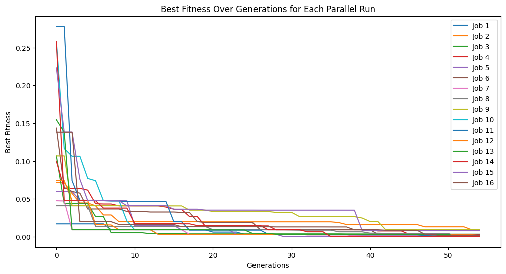
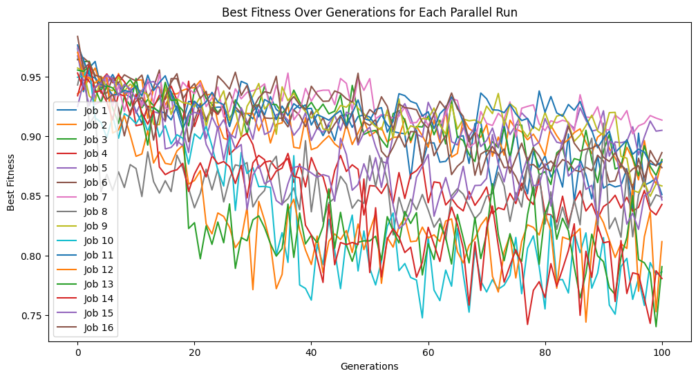
Setting elitismRate=0 will make it so no individuals are preserved across generations, so progress is not guaranteed. This can be observed by seeing that the evolution trace is no longer monotonic.
#Generate models
models=sgp.parallelEvolve(inputData,response,tracking=True, elitismRate=0)
Running parallel evolution with 16 jobs.
popSize#
We can control the population size using the popSize option. By default we target a population of 300 models. It may be the case that we want to increase the size to allow for more diverse models to exist, or we may want to make it easier to progress deeper into evolution by using smaller populations and making it less computationally expensive to evaluate each generation.
#Define a function to generate data
def demoFunc(x,y):
    return np.sin(x)/np.cos(y) * y**2
#Generate data
inputData=np.array([np.random.randint(1,10,10),np.random.randint(1,10,10)])
response=demoFunc(inputData[0],inputData[1])
Below we set a very small population size of 10 models. We can see that it makes it through the set number of generations very quickly, but due to a lack of diversity, we don’t get to very good models.
#Generate models
models=sgp.parallelEvolve(inputData,response,tracking=True, popSize=10)
Running parallel evolution with 16 jobs.
Looking at the population, we can see there are very few models.
sgp.plotModels(models)
Using a population size of 1000 makes the evolution much slower, but we can see we arrived at much better models since the population contained more potentially useful genetic material to use.
#Generate models
models=sgp.parallelEvolve(inputData,response,tracking=True, popSize=1000)
Running parallel evolution with 16 jobs.
Looking at the population, we can see that there are many more models
sgp.plotModels(models)
maxComplexity#
We can control the max complexity allowed in the search space by setting the maxComplexity option. Complexity is determined by counting the total combined lengths of the operator and data stacks.
#Define a function to generate data
def demoFunc(x,y):
    return np.sin(x)/np.cos(y) * y**2
#Generate data
inputData=np.array([np.random.randint(1,10,10),np.random.randint(1,10,10)])
response=demoFunc(inputData[0],inputData[1])
#Generate models
models=sgp.parallelEvolve(inputData,response,tracking=True, maxComplexity=10)
Running parallel evolution with 16 jobs.
After search, some post processing steps may occur that could increase the model size slightly, so we can see some models a bit over the max complexity of 10.
sgp.plotModels(models)
We can crank the complexity limit up to 1000 to see what happens.
#Generate models
models=sgp.parallelEvolve(inputData,response,tracking=True, maxComplexity=1000)
Running parallel evolution with 16 jobs.
Setting a max complexity does not mean we will get models up to that complexity. The search will prioritize simpler accurate models, so unless it is necessary, you won’t see many models near a very high complexity limit. As we can see below, the models are hardly more complex than when we set the max complexity to 10.
sgp.plotModels(models)
align#
The align option is a binary setting which determines if models will undergo linear scaling at the end of evolution. Since the default accuracy metric is \(R^2\), there is no guarantee that the model will have the best scaling and translation coefficient, so this scaling step is necessary to align the model with the training data. By default this option is set to True, but if a different accuracy metric is being used, such as RMSE, it may not be necessary to use the alignment.
#Define a function to generate data
def demoFunc(x,y):
    return 5*x*y+2
#Generate data
inputData=np.array([np.random.randint(1,10,10),np.random.randint(1,10,10)])
response=demoFunc(inputData[0],inputData[1])
Lets first show what happens when we set align=False. We can see that we get to a model with essentially 0 error.
#Generate models
models=sgp.parallelEvolve(inputData,response,tracking=True, align=False)
Running parallel evolution with 16 jobs.
When we look at the model though, we can see that it is clearly not the same as the function used to generate the data. It has a similar form, but the constants are wrong.
sgp.printGPModel(models[0])
Now when we set align=True we again get to a model with essentially 0 error.
#Generate models
models=sgp.parallelEvolve(inputData,response,tracking=True, align=True)
Running parallel evolution with 16 jobs.
When we look at the best model though, we can see that now it has the same form and constants as the formula used to generate the data.
sgp.printGPModel(models[0])
initialPop#
We can seed the evolution by providing an initial population. Assuming we have previously generated models from other searches, this can allow us to transfer previously learned patterns into our current search to kick start the process.
#Define a function to generate data
def demoFunc(x,y):
    return np.sin(x)/np.cos(y) * y**2
#Generate data
inputData=np.array([np.random.randint(1,10,10),np.random.randint(1,10,10)])
response=demoFunc(inputData[0],inputData[1])
We first need to run an initial evolution to get a population to feed into another search.
#Generate models
models=sgp.parallelEvolve(inputData,response,tracking=True)
Running parallel evolution with 16 jobs.
We can see that the error trace begins where the previous search left off since the new search started with the previously evolved models.
#Generate models
models=sgp.parallelEvolve(inputData,response,tracking=True,initialPop=models)
Running parallel evolution with 16 jobs.
We can do this process as many times as we want to continue iteratively improving our models.
#Generate models
models=sgp.parallelEvolve(inputData,response,tracking=True,initialPop=models)
Running parallel evolution with 16 jobs.
timeLimit#
Often, we are constrained by time when performing our analysis or modeling so we care about controlling the runtime of the search. We can set the max runtime by setting the timeLimit option to the max number of seconds and setting the capTime option to True.
#Define a function to generate data
def demoFunc(x,y):
    return np.sin(x)/np.cos(y) * y**2
#Generate data
inputData=np.array([np.random.randint(1,10,10),np.random.randint(1,10,10)])
response=demoFunc(inputData[0],inputData[1])
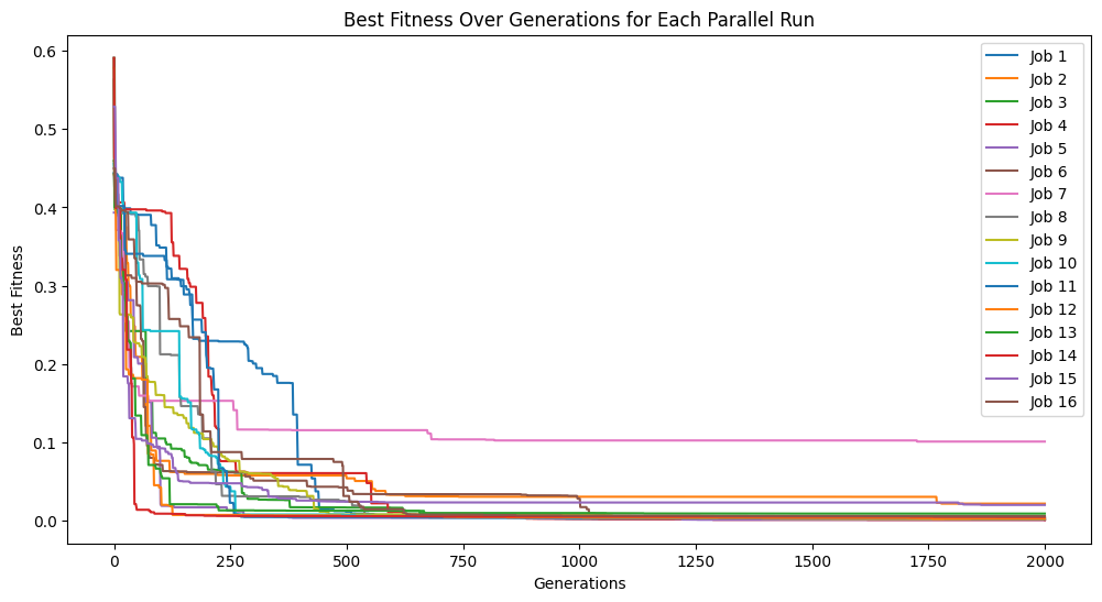
By default, the search will run until a set number of generations has been completed. Depending on the problem, the actual runtime to complete a set number of generations can vary significantly and can be difficult to predict in advance. Therefore, a runtime limit is often more practical. The below example does not have a time limit and will run until it completes 2,000 generations. This process took about ~5 minutes to run.
#Generate models
models=sgp.parallelEvolve(inputData,response,tracking=True,generations=2000)
Running parallel evolution with 16 jobs.
Below we set timeLimit=30 and capTime=True to stop the search when we reach 30 seconds of runtime.
#Generate models
models=sgp.parallelEvolve(inputData,response,tracking=True,generations=10000, timeLimit=30, capTime=True)
Running parallel evolution with 16 jobs.
If the number of generations are completed before the time limit the search will terminate. Below we can see that the 100 generation completes before the time limit of 60 seconds.
#Generate models
models=sgp.parallelEvolve(inputData,response,tracking=True,generations=100, timeLimit=60, capTime=True)
Running parallel evolution with 16 jobs.
tourneySize#
We can control the tounament size used in selection by setting the tourneySize option. Larger tournament sizes will make the search more greedy, while smaller sizes will make it less greedy.
#Define a function to generate data
def demoFunc(x,y):
    return np.sin(x)/np.cos(y) * y**2
#Generate data
inputData=np.array([np.random.randint(1,10,10),np.random.randint(1,10,10)])
response=demoFunc(inputData[0],inputData[1])
The below shows an example where we set the tournament size to 5 models.
#Generate models
models=sgp.parallelEvolve(inputData,response,tracking=True,tourneySize=5)
Running parallel evolution with 16 jobs.
Below we increase the tournament size to 30 models.
#Generate models
models=sgp.parallelEvolve(inputData,response,tracking=True,tourneySize=30)
Running parallel evolution with 16 jobs.
tracking#
The tracking option is a binary setting that allows us to visualize the evolution trace to see how the model search progressed. It has been set to True throughout most of the examples above to show the evolutionary search progress. If you don’t want the trace plot cluttering up your notebook space or if you are calling the function headless, you may want to set it to False.
#Define a function to generate data
def demoFunc(x,y):
    return np.sin(x)/np.cos(y) * y**2
#Generate data
inputData=np.array([np.random.randint(1,10,10),np.random.randint(1,10,10)])
response=demoFunc(inputData[0],inputData[1])
Below we can see that by setting tracking=False, nothing is displayed when running evolve.
#Generate models
models=sgp.parallelEvolve(inputData,response,tracking=False)
Running parallel evolution with 16 jobs.
Setting tracking=True below makes it so when we run evolve we see the evolution trace.
#Generate models
models=sgp.parallelEvolve(inputData,response,tracking=True)
Running parallel evolution with 16 jobs.
modelEvaluationMetrics#
The choice of fitness objectives can have a significant impact on the success of search, so it is useful to be able to change these. These can be changed by providing them as a list to modelEvaluationMetrics. By default, modelEvaluationMetrics=[fitness,stackGPModelComplexity] is used, where fitness is \(R^2\) and stackGPModelComplexity is combined stack length. A list of any length can be supplied. Each function in the list will be given as arguments the model, input data, and response vector in that order.
#Define a function to generate data
def demoFunc(x,y):
    return np.sin(x)/np.cos(y) * y**2
#Generate data
inputData=np.array([np.random.randint(1,10,10),np.random.randint(1,10,10)])
response=demoFunc(inputData[0],inputData[1])
Below we define RMSE as a fitness function
#Define new fitness objective (RMSE)
def rmse(model, inputData, response):
    predictions = sgp.evaluateGPModel(model, inputData)
    return np.sqrt(np.mean((predictions - response) ** 2))
Below we use rmse and stackGPModelComplexity as our fitness objectives.
#Generate models
models=sgp.parallelEvolve(inputData,response,tracking=True,modelEvaluationMetrics=[rmse,sgp.stackGPModelComplexity])
Running parallel evolution with 16 jobs.
We can see the form of the best model found.
sgp.printGPModel(models[0])
Now we can compare the best model’s predictions and the true response data.
sgp.plotModelResponseComparison(models[0],inputData,response)
Now we change to use the default settings which uses fitness and stackGPModelComplexity.
#Generate models
models=sgp.parallelEvolve(inputData,response,tracking=True,modelEvaluationMetrics=[sgp.fitness,sgp.stackGPModelComplexity])
Running parallel evolution with 16 jobs.
Now we can see the form of the best model found during search.
sgp.printGPModel(models[0])
Now we compare the model’s predictions to the true response values.
sgp.plotModelResponseComparison(models[0],inputData,response)
If we only want a single objective search, we can supply just one objective. Notice that the search takes longer since there is no constraint on model size, so models will become larger and more expensive to evaluate.
#Generate models
models=sgp.parallelEvolve(inputData,response,tracking=True,align=False, modelEvaluationMetrics=[sgp.fitness])
Running parallel evolution with 16 jobs.
We can confirm this by looking at the size of models. We can see that many are fairly large.
# Update the model quality using standard objectives so we can create the standard model quality plot
[sgp.setModelQuality(mods, inputData, response) for mods in models]
sgp.plotModels(models)
We may also be interested in optimizing on a 3D front. In this case, we can supply a list of 3 objectives.
#Generate models
models=sgp.parallelEvolve(inputData,response,tracking=True,modelEvaluationMetrics=[sgp.fitness,sgp.stackGPModelComplexity, rmse])
Running parallel evolution with 16 jobs.
The plotModels function will only plot with respect to the first two objectives.
sgp.plotModels(models)
We can see the embedded quality of a model by grabbing the end of it. The order of objectives is the same as the order supplied. In this case fitness, stackGPModelComplexity, and rmse.
models[0][-1]
[np.float64(0.02699349215824387), 27, np.float64(7715410.079728199)]
dataSubsample#
In scenarios where a data set is very large, it may cause training to be prohibitively slow. You could subsample the data set before passing it to the model training, but then the models are underinformed during training since they do not get the opportunity to learn about all the data. By setting dataSubsample=True you can supply the entire training set and then during evolution the set will be randomly sampled in each generation. The constant shuffling of data allows the models to learn from the whole data set while keeping training efficient since only a small set is used in each generation.
#Define a function to generate data
def demoFunc(x,y):
    return np.sin(x)/np.cos(y) * y**2
#Generate data
inputData=np.array([np.random.randint(1,10,1000000),np.random.randint(1,10,1000000)])
response=demoFunc(inputData[0],inputData[1])
Running the code below, we can see it takes quite a while to train when using 1,000,000 training points.
models=sgp.parallelEvolve(inputData,response,tracking=True)
Running parallel evolution with 16 jobs.
sgp.printGPModel(models[0])
When we enable data subsampling, we can see the training completes much faster. We can also notice that the training fitness no longer monotonically decreases since the training points used to determine fitness are constantly being resampled.
samplingModels=sgp.parallelEvolve(inputData,response,tracking=True,dataSubsample=True)
Running parallel evolution with 16 jobs.
In a scenario where you are constrained by time, the subsampling can make a huge difference. For example, below we constrain the search to 10 seconds and do not subsample. We can see that we make it through very few generations and the model quality does not improve very much.
timeConstrainedModels=sgp.parallelEvolve(inputData,response,tracking=True,dataSubsample=False,capTime=True,timeLimit=10)
Running parallel evolution with 16 jobs.
Below is the plot showing the quality of the models in the population.
sgp.plotModels(timeConstrainedModels)
Now if we have the same time constraint but instead allow subsampling, we can make it through many more generations in that time. This also allows us to potentially find better models since the search is deeper.
timeConstrainedSampledModels=sgp.parallelEvolve(inputData,response,tracking=True,dataSubsample=True,capTime=True,timeLimit=10)
Running parallel evolution with 16 jobs.
Below is a plot showing the quality of models in the population.
sgp.plotModels(timeConstrainedSampledModels)
samplingMethod#
In scenarios where a data set is very large, it may cause training to be prohibitively slow. You could subsample the data set before passing it to the model training, but then the models are underinformed during training since they do not get the opportunity to learn about all the data. By setting dataSubsample=True you can supply the entire training set and then during evolution the set will be randomly sampled in each generation. The constant shuffling of data allows the models to learn from the whole data set while keeping training efficient since only a small set is used in each generation. By default, when data sampling is active, the randomSubsample strategy is used. This strategy selects a new random sample every generation and the sample size remains the same across all generations.
Note: Regardless of the subsampling strategy, before models are returned, all models are evaluated on the full training set so that the returned fitness values are representative of the model quality on the entire training set.
#Define a function to generate data
def demoFunc(x,y):
    return np.sin(x)/np.cos(y) * y**2
#Generate data
inputData=np.array([np.random.randint(1,10,1000000),np.random.randint(1,10,1000000)])
response=demoFunc(inputData[0],inputData[1])
Here we use the randomSubsample strategy that randomly chooses a subset of the full training set each generation.
samplingModels=sgp.parallelEvolve(inputData,response,tracking=True,dataSubsample=True,samplingMethod=sgp.randomSubsample,capTime=True,timeLimit=10)
Running parallel evolution with 16 jobs.
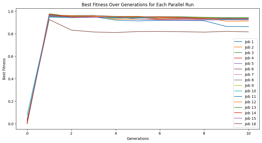
Here we use generationProportionalSample to start with a very small sample size and increase as we progress through generations. Note that the big jump in fitness is a result of starting with just 3 training points which is very easy to overfit, thus a near perfect fitness on the 3 point training set.
samplingModels=sgp.parallelEvolve(inputData,response,tracking=True,dataSubsample=True,samplingMethod=sgp.generationProportionalSample,capTime=True,timeLimit=10)
Running parallel evolution with 16 jobs.
It is also possible to use user defined sampling methods. For example, here we implement a inverse generation proportional sampling. While it likely wouldn’t be useful to do this, we can use this to illustrate how this can be done.
def inverseGenerationProportionalSample(fullInput,fullResponse,generation,generations):
    prop=(generations-generation)/generations
    sampleSize=int(prop*len(fullResponse))
    if sampleSize<3:
        sampleSize=3
    indices=np.random.choice(len(fullResponse),size=sampleSize,replace=False)
    return fullInput[:,indices],fullResponse[indices]
We will make the training set a bit smaller to better showcase the impact here.
inputData=np.array([np.random.randint(1,10,10000),np.random.randint(1,10,10000)])
response=demoFunc(inputData[0],inputData[1])
inverseSamplingModels=sgp.parallelEvolve(inputData,response,tracking=True,dataSubsample=True,samplingMethod=inverseGenerationProportionalSample,capTime=True)
Running parallel evolution with 16 jobs.